The Haunt Roll in Betrayal Games

I'll get to the Betrayal games in a minute, but let me share some background for how I'm approaching it.

There was a recent question on BoardGameGeek that asked about a mechanic for finding a spy amidst a group of senators. The proposal was to use a bag with 11 tokens, 2 of which are spy tokens, with the remaining 9 being senators. Both spy tokens need to be drawn to find the spy.

I would like the average resolution to be about 6-7 attempts, hopefully landing in the neighborhood of 4-9 attempts, beyond some extreme flukes.

First, let me say that I love the framing here in terms of the desired average and extremes. We can evaluate the mechanic much better with a design criteria as described above.

As to the problem, we can simplify the problem by turning it around, which avoids having to consider the combinatorics of order. This approach is similar to how I've solved the game length in High Society. Let's analyze the problem as if the order the chits is known or determined ahead of time (even though it isn't). The question then becomes, what is the probability that the second spy chit is in round $r$ counting from the front? That's the same as looking for the first spy chit from the back of the line. For the last round,$r=9$, that's easy,

\begin{align} P(r=9) = \frac{2}{11}, \end{align}

as there are 2 spies out of 11 total tokens. Let's count this as round $n=1$ from the back.

\begin{align} P(n=1) = \frac{2}{11} \end{align}

For earlier rounds, we must have drawn all senators "first" (again, we're starting at the back). The probability of drawing a senator in a round $n$ from the back is based on the number of tokens that weren't drawn yet. If we've yet to draw a spy, in round $n$, there are $11-(n-1)=12-n$ total tokens. Two of them are spies, so $12-n-2$ are spies. Thus the probability of drawing a senator in round $n$ (from the back) given no previous spies is as follows.

\begin{align} P(\text{senator in round } n | \text{ no spies in rounds} < n) & = \frac{11 - (n-1) - 2}{11 - (n-1)} \\ &= \frac{10-n}{12-n} \end{align}

So first $\frac{9}{11}$, then $\frac{8}{10}$, and so on. Similarly, the probability of drawing the "first" spy in round $n$ from the back is,

\begin{align} P(\text{spy in round } n | \text{ no spies in rounds} < n) & = \frac{2}{11 - (n-1)} \\ &= \frac{2}{12-n}. \end{align}

We can combine the above in order to get the probability of finding a spy in round $n$. To be able to write the probabilities in a more compact way, such that we can fit our equations on one line, let's make use of the following events.

\begin{align} S_n &= \text{senator in round } n \\ Y_n &= \text{spy in round } n \end{align}

We can rewrite the above probabilities using these events.

\begin{align} P\left(S_n \:\middle\vert\: \bigcap_{i<n} S_i\right) &= P(\text{senator in round } n \mid \text{no spies in rounds} < n)\\ P\left(Y_n \:\middle\vert\: \bigcap_{i<n} S_i\right) &= P(\text{spy in round } n \mid \text{no spies in rounds} < n) \end{align}

Here $\bigcap_{i<n} S_i$ refers to the intersection of all events $S_i$ when $i<n$. Basically, that means $S_1$, $S_2$, $\ldots$, $S_{n-2}$, and $S_{n-1}$ all occur. Note that because senators and spies are mutually exclusive and the only options,

\begin{align} P(Y_n) = 1- P(S_n). \end{align}

Using this more compact notation, we can combine our previous equations to get the total probability of drawing the first spy in round $n$ from the back.

\begin{align} P(Y_n) &= P\left(Y_n \:\middle\vert\: \bigcap_{i<n} S_i\right) \cdot P\left(\bigcap_{i < n} S_i\right) \end{align}

Recall that $P(S_i)$ depends on what was previous drawn, meaning that $S_i$ are not independent. Because of this, we cannot simply break up $P\left(\bigcap_{i < n} S_i\right)$ as a product of the probabilities.

\begin{align} P\left(\bigcap_{i < n} S_i\right) &\neq \prod_{i=1}^n P(S_i) \\ \end{align}

Instead, we use the conditional probabilities that we found earlier.

\begin{align} P(Y_n) &=P\left(Y_n \:\middle\vert\: \bigcap_{i<n} S_i\right) \cdot\prod_{i=1}^n P\left(S_i \:\middle\vert\: \bigcap_{k<i} S_k\right) \\ &= \frac{2}{12-n}\frac{9}{11} \cdot \frac{8}{10} \cdot \ldots \cdot \frac{10-(n-1)}{12-(n-1)} \\ &= \frac{2 \cdot 9 \cdot 8 \cdot \ldots \cdot (10-(n-1))}{11 \cdot 10 \cdot \ldots \cdot (12-n)} \\ &= 2 \cdot \frac{9!}{11!} \cdot \frac{(12-(n+1))!}{(10-n)!} \end{align}

At this point, we can turn things back around to count from the front. We know that $n=1$ is equivalent to $r=11$ and $n=11$ is equivalent to $r=1$. From this we can write the equations defining the relationship between the number of rounds from the front, $r$, and the number of rounds from the back, $n$.

\begin{align} n = 12-r \end{align}

Thus the probability of finding the spy chit in round $r$ is as follows.

\begin{align} P(\text{spy revealed in round } r) &= P(Y_{12-r}) \\ &= 2 \cdot \frac{9!}{11!} \cdot \frac{(12-(12-r+1))!}{(10-(12-r))!}\\ &= 2 \cdot \frac{9!}{11!} \cdot \frac{(r-1)!}{(r-2)!} \\ &= 2 \cdot \frac{9!}{11!} \cdot (r-1) \\ &= \frac{2}{11\cdot 10} \cdot (r-1) \end{align}

The result of this equation is shown in Figure 1, which shows a linearly increasing probability as each new token is drawn, starting with a probability of 0 in round 1. This makes sense, as the second spy token must be drawn to actually find the spy. A numerical check confirms that the values for all value $r$ sum to 1. As clearly shown in the plot, this favors the last rounds, which does not match the desired properties.

Figure 1: Probability of finding the spy

Now, let's turn to the haunt roll mechanics found in the various Betrayal games, including Betrayal at the House on the Hill, Betrayal at Balder's Gate, Betrayal Legacy, and Betrayal at Mystery Mansion. We'll actually set the legacy version aside, as the legacy aspects of the game can influence the roll.

In the original game (Betrayal at the House on the Hill), each time an omen is drawn the active player rolls 6 dice and if the result is less than the number of omen cards then the haunt starts (the example in the rulebook actually says equal to or less than number of omen cards, which I'll assume is an error). The dice in all betrayal games are the same: custom six-sided dice with two sides each of 0, 1, and 2. This means the probability mass function (pmf) of each die is $1/3$ for values on the dice, and $0$ elsewhere. We'll denote the result of one of the betrayal dice as a random variable $D$ with pmf $f_D(d)$.

\begin{align} f_D(d) = \begin{cases} \frac{1}{3} \quad & d \in {0, 1, 2} \\ 0 \quad &\text{else} \end{cases} \end{align}

We can get the pmf of the entire hunt roll of six dice, $f_H(h)$ by convolving the pmf of each die with itself enough times to account for the six dice that a player rolls.

\begin{align} f_H(h) = f_D(h) * f_D(h) * f_D(h) * f_D(h) * f_D(h) * f_D(h) \end{align}

Because convolution is associative, we don't have to worry about the order of the convolutions. The result is shown in calculation in Figure 2. We get what we expect after convolving a reasonable number (even if it is only six here) of independent identically distributed (i.i.d.) random variables, which is a roughly Gaussian, or normal-looking distribution.  (Due to the Central Limit Theorem. There are probably some comments I should be making about whether them being identically distributed matters here, but I'll omit them for ease and brevity.) We expect a minimum value of 0 and maximum value of 12, each corresponding to the extreme values on all dice. These are possible, but with low probability. The distribution is also symmetric.

Figure 2: Probability mass function of haunt roll

By computing the cumulative distribution (CDF) of the haunt roll result, $F_H(h)$, we can easily compute the probability that the haunt starts in any given round. Finding the CDF is a straightforward computation based on the pmf.

\begin{align} F_H(h) &= P(H \leq h) \\ &= \sum_{i=0}^h f_H(i) \end{align}

Figure 3: Cumulative distribution function of haunt roll

Note that here, the minimum possible value on a haunt roll is 0. The resulting CDF is plotted in Figure 3. Because the haunt starts whenever the haunt roll is less than the number of omens drawn, the probability of a haunt being triggered when making a haunt roll is equal to the CDF evaluated at one less than the number of omens, $o$.

\begin{align} P(\text{haunt starts} \mid o \text{ omens}) = F_H(o-1) \end{align}

The next step is to assemble the probability distribution of the number of omens drawn before the haunt starts. We use the distribution of the haunt roll to do this, noting that we only consider drawing more omens if the haunt starts. Therefore, the probability that the number of omens when the haunt starts, $O$, is 1 is equal to the probability that we roll less than 1 on the first haunt roll.

\begin{align} f_O(1) &=P(O=1)\\ &= F_H(1-1)\\ & = F_H(0)\\ &=f_H(0)\\ &=f_D(0)^6\\ & \left( \frac{1}{3} \right)^6 \\ &\approx 0.00137 \end{align}

In this case, as shown above, the probability shakes out to the probability of rolling 0 on all six haunt dice, which occurs with a probability of about 0.00137.

When looking at the probability that $O>1$, we must consider the result of all previous haunt rolls. That is, we only make a haunt roll with $o$ omens, where $o>1$, if all previous haunt rolls failed to start the haunt.

\begin{align} P(\text{make haunt roll with $o$ omens}) &= 1 - P(O < o)\\ &= 1- F_O(o-1)\\ & 1 - \sum_{i=0}^{o-1}f_O(i) \end{align}

This gives us an equation to compute the distribution of $O$ where we can compute each term one at a time, using the one term to compute the next.

\begin{align} f_O(o) &= \left ( 1 - \sum_{i=0}^{o-1}f_O(i) \right) \cdot F_H(o-1) \end{align}

Now that we've gone all the way through this exercise, we can turn to the other versions of the game. Betrayal and Balder's Gate and Betrayal at Mystery Mansion both function similarly (though the latter game uses the term clue instead of omen, it functions the same). Instead of rolling a constant number of dice and adjusting the target number, the number of dice rolled is equal to the number of omen cards drawn and a constant target number is used. In Balder's Gate, if the haunt roll is 6 or higher the haunt starts, whereas Mystery Mansion uses a threshold of 5 or higher.

To compute the distribution of dice, we can use a similar method as above, but varying the number of haunt dice pmfs which are convolved. The resulting pmfs and CDFs are plotted in Figures 4 and 5.

Figure 4: Probability mass function of haunt roll by omen

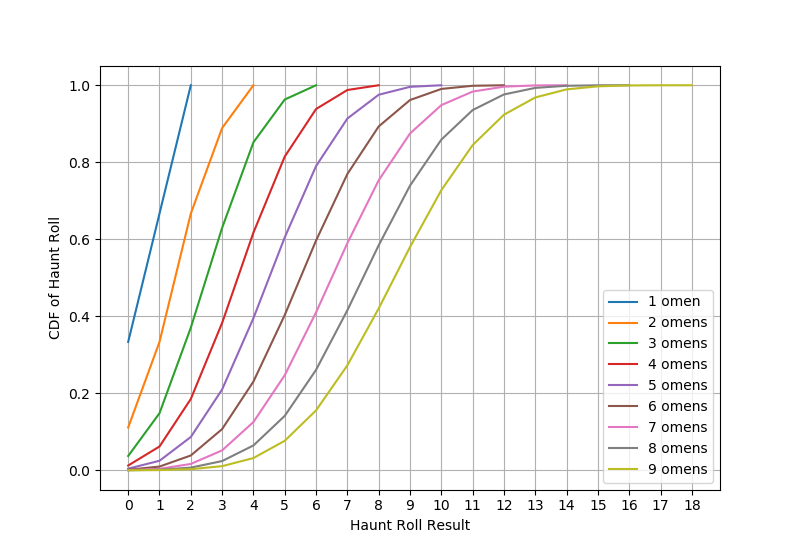Figure 5: Cumulative distribution function of haunt roll by omen

We can reuse the same equation to find the pmf and CDF of the number of omens drawn before the haunt starts for the three games, which are plotted in Figures 6 and 7. We can note a couple differences. Most evident is that each iteration on the game tends to make the haunt start sooner, as shown most clearly in the CDFs. Second, the possibility of a very early haunt with the original game, with only 1 or 2 drawn, has been completely eliminated in Balder's Gate and Mystery Mansion. For the later games, rolling one or two dice is insufficient to get a sum or 5 or 6 to trigger the haunt. On the other hand, these games have a non-zero probability of an arbitrarily long game according to the probabilities shown. Mystery Mansion has a special rule that the haunt always starts after the 9th omen (clue) card is drawn.

Figure 6: Probability of triggering the haunt when drawing current omen

Figure 7: Cumulative probability of triggering the haunt

We could modify the dice so that they naturally provide both an upper and lower bound, as originally desired for the spy search mechanism, by using a similar mechanism to the later Betrayal games but having a non-zero minimum value on the dice. Doing this sets a maximum number of turns needed for the search, equal to the ratio between the target sum and the minimum value on the dice.

Recall that we want between 4 and 9 searches, averaging 6-7. Let's use a minimum value of 1 on the dice and decide on the number of values to include to achieve the properties above. With a minimum of 1 and max 9 rounds, the target sum must be 9. To prevent 3 searches from being successful, there must be at most 2 sides on the dice. This gives the distributions functions shown in Figures 8 and 9. While these center more on 6 searches, they demonstrate the feasibility of this type of mechanism. The particular type of dice and target numbers can be adjusted to get the desired probability properties.

Figure 8: Probability of finding the spy in the current round (pmf)

Figure 9: Cumulative probability of finding the spy by round (CDF)