Monday, April 27, 2020

Are you a Cylon in Battlestar Galactica?

Note: there are errors contained in this post.  See errata here.

Of course I'm not. A few variables complicate this. Foremost is that it depends on when in the game you're asking about. In most cases, each player receives one loyalty card at the beginning of the game, and second one in the middle of the game during the sleeper agent phase. However, two characters (Baltar and Boomer) draw an extra loyal card (at the beginning and middle of the game, respectively) and each add an extra human loyalty card into the mix. It also depends on how many players there are, and thus how many Cylon cards there are. Having one or more Cylon cards makes you a Cylon.

Let's consider the five player case (two Cylons), and assume Baltar and Boomer are not involved. Thus, there are ten loyalty cards in use, eight human and two Cylon. I'll get dealt two loyalty card throughout the game. During the first half, the probability that I'm a Cylon is,
\begin{align}
P(\text{Cylon}) = \frac{2}{10}.
\end{align}
(This is assuming that we don't count drawing a Cylon card later as having been a Cylon all along. This assumption is not necessarily valid on two fronts. First, in the fiction, characters do not become Cylons. Second, if the loyalty deck were already shuffled at the beginning of the game and the order in which they will be dealt determined, then my fate as human or Cylon would be sealed already—ignoring a revealed Cylon giving me a Cylon card—I just don't know it yet.)
There are two cards out of the ten possible that could make me a Cylon at the beginning of the game. Next, let's consider the entirety of the game. Since I could be a Cylon card at the beginning, middle, or both, it's easier to frame being a Cylon as being mutually exclusive as being human. That is,
\begin{align}
P(\text{Cylon}) + P(\text{human}) = 1.
\end{align}
Which we can rearrange to find the probability of being a Cylon.
\begin{align}
P(\text{Cylon}) = 1 - P(\text{human})
\end{align}
To be human, I must get two human cards.
\begin{align}
P(\text{human}) &= P(\text{first human} \cap \text{second human})
\end{align}
Here the probability $P(\text{first human}\,  \cap \, \text{second human})$ is the probability that my first card is human and my second card is human. The symbol $\cap$ is for intersection, which essentially means and. These events are not independent, so we express the joint probability as follows.
\begin{align}
P(\text{human}) &= P(\text{first human}) \cdot P(\text{second human} | \text{first human})
\end{align}
The probability of getting the first human card is in some sense the opposite of getting a Cylon card as my first card.
\begin{align}
P(\text{first human}) &= 1 - \frac{2}{10} \\
P(\text{first human}) &= \frac{8}{10}
\end{align}
We can also see this as there are eight human cards out of ten total loyalty cards.

The second term is one of conditional probability: the probability that the second card is human given the fact that the first card is human. Here the vertical bar, $|$,  means given. Knowing whether the first card is human or not affects the probability of the second card. If I don't know anything about the first card, the probability is the same.
\begin{align}
P(\text{second human}) &= \frac{8}{10}
\end{align}
Given that I've gotten a human card first, there are seven human cards left out of a total of nine loyalty cards.
\begin{align}
P(\text{second human} | \text{first human}) &= \frac{7}{9}
\end{align}
Or given that I got a Cylon card first, there would be eight human cards left out nine total.
\begin{align}
P(\text{second human} | \text{first Cylon}) &= \frac{8}{9}
\end{align}
We can now combine the results to find the probability that I'm a Cylon.
\begin{align}
P(\text{Cylon}) &= 1 - P(\text{first human}) \cdot P(\text{second human} | \text{first human}) \\
&= \frac{8}{10} \cdot \frac{7}{9} \\
&= \frac{56}{90} = \frac{28}{45} = \frac{2\cdot 2 \cdot 7}{3\cdot 3\cdot 5} \\
&\approx 0.622
\end{align}
What we've done is correct, but the result is not useful because you always have some information; you know your own card(s). There are three cases: you have no Cylon card, you have one Cylon card, and you have two Cylon cards. The last case is the simplest to dispatch. Since there are only two Cylon cards and you have them both, I have no chance of being a Cylon.
\begin{align}
P(\text{I'm Cylon} | \text{you have two Cylon cards}) = 0
\end{align}
For the other cases, where you have zero or one Cylon cards, can be computed as variations on the earlier analysis. I leave this as an exercise for the reader.

You may gain additional information at some point in the game though. There are a number of scenarios in which you may be able to randomly look at one of my loyalty cards. Interestingly, it matters whether you do this before or after the sleeper agent phase.

Let's consider the case where you're human and earlier in the game, before the sleeper agent phase, you got to look at my (then) only loyalty card. Then, the only possibility of me being a Cylon is that I get one for my second loyalty card. You've seen three human cards, two of yours and one of mine. Leaving seven out of ten about whose location you know nothing. Thus, the probability that I'm a Cylon is,
\begin{align}
P(\text{second Cylon} | \text{first human}) &= \frac{2}{7} \approx 0.286.
\end{align}
However, if you saw one of my two cards after the sleeper agent phase, the probability is different because while you know that I don't have two Cylon cards, you don't know whether you looked at my first or second loyalty card. We'll find the probabilities ignoring what you saw first. You know that you have two human cards, so eight cards are unknown. The probability that I am human given that you are human is,
\begin{align}
P(\text{human}) &= \frac{6}{8}\cdot\frac{5}{7} \approx 0.536.
\end{align}
The probability that I have one Cylon card and one human card is the sum of the probability of two cases. In the first, I get a Cylon card then a human card. In the second, I get a human card then a Cylon card. Calculating these probabilities is very similar to the earlier calculations
\begin{align}
P(\text{human then Cylon}) &= P(\text{first human}) \cdot P(\text{second Cylon} | \text{first human}) \\
&= \frac{6}{8} \cdot \frac{2}{7} \\
P(\text{Cylon then human}) &= P(\text{first Cylon}) \cdot P(\text{second human} | \text{first Cylon}) \\
&= \frac{2}{8} \cdot \frac{6}{7} \\
\end{align}
We can add these up since they are disjoint. As you can see, the probabilities are equal.
\begin{align}
P(\text{1 Cylon}) &= P(\text{human then Cylon}) + P(\text{Cylon then human}) \\
&=  \frac{6}{8} \cdot \frac{2}{7} + \frac{2}{8} \cdot \frac{6}{7}\\
&= 2 \cdot  \frac{6}{8} \cdot \frac{2}{7} \\
& \approx 0.429
\end{align}
The probability that I'm Cylon given that you saw I have one human card involves scaling the probability that I have one Cylon card  by the probability that I have at least one human card.
\begin{align}
P(\text{Cylon} | \geq 1 \text{ human card}) &= \frac{P(\text{1 Cylon})}{P( \geq 1 \text{ human card})} \\
&= \frac{P(\text{1 Cylon})}{P(\text{1 Cylon}) + P(\text{human})} \\
&= \frac{  2 \cdot  \frac{6}{8} \cdot \frac{2}{7} } { 2 \cdot  \frac{6}{8} \cdot \frac{2}{7} +  \frac{2}{8} \cdot \frac{6}{7}} \\
&= \frac{  2 \cdot  6 \cdot 2 } { 2 \cdot  6 \cdot 2 +  2 \cdot 6} \\
&= \frac{  6 \cdot 2 } {  6 \cdot 2 +  6} \\
&= \frac{  6 \cdot 2 } {  6 \cdot 3 } \\
&= \frac{  2 } {  3 } \\
& \approx 0.667
\end{align}
Note that this is substantially higher than if you had seen my first loyalty card. If you think about these two scenarios vaguely, they seem like they may be the same. In both cases you saw that one of my loyalty cards is human. However, in the first case you saw my first card, which is not specified in the second case. In the second case, all we know is that at least one of my cards is human. This is related to the woman in the park with the two kids problem referenced in our discussion of Catan. The lack of ambiguity is especially clear in the Cylon probabilities discussed here. Differentiating the two cases is worth understanding, especially when given information more abstractly without the origin of that information made clear.

Monday, April 20, 2020

Is there a flaw in Savage Worlds?

You might ask:
I've read that there's a flaw in the way the dice work in Savage Worlds. Can you explain that?
Sure... Let me first say that I disagree that there's a flaw; the designers made a valid design tradeoff (though, just as with my Battletech partial cover analysis, I don't have any knowledge of the actual decision-making process). Let's go through the claim and the math behind it.

In Savage Worlds, in general, you're rolling a die and trying to get 4 or higher. (Getting higher multipliers may also be good, but let's keep things simple.) You roll a different size die depending on what skill or ability you're rolling. You may roll 1d4, 1d6, 1d8, 1d10, or 1d12. (You'll also roll a "wild die'' with this, a 1d6, which we'll ignore for now.) If you roll the maximum possible for the die you are rolling, you get to roll again and add the results. That is, if you roll $N$ on 1d$N$, you roll 1d$N$ again, and take $N$ plus the result of the second roll as your total result. You can keep doing this as long as you keep rolling the maximum. So you if you are rolling 1d6, and roll 6, 6, 6, 3, then your total result is 21.

Wow, doesn't this mean that you can roll infinitely high? Yes.

So what's the probability distribution look like? Let's continue to work with 1d6 for the moment. If we roll 1–5, we know the probability is $1/6$. Let's say our total result is $Y$.
\begin{align}
P(Y=y) = \frac{1}{6} \quad y \in \{1,2,\cdots,5\}
\end{align}
Interestingly, the probability of getting a $Y= 6$ is zero. This is because when you roll a 6 you roll another die and add the result. The minimum you get on the second die is 1. The probability of getting 7–11 is,
\begin{align}
P(Y=y) ,\ y \in \{7,8,\cdots,11\} &= P(\text{first roll 6}) \cdot P(\text{then roll }y-6) \\
& = P(Y_1 = 6) \cdot P(Y_2 = y_2) ,\ y_2 = y-6 \\
& = \frac{1}{6} \cdot \frac{1}{6} \\
& = \frac{1}{36} \approx 0.0278.
\end{align}
Here we've introduced $Y_1$ and $Y_2$ to simplify our equations, where $Y_i$ refers to the $i$-th roll of the die to determine the total sum. Most of the time you'll only roll once, unless you get a 6.  Similarly to the $Y=6$ case, $P(Y=12) = 0$. And then
\begin{align}
P(Y=y) &,\ y \in \{13,14,\cdots,17\} \\
& = P(Y_1 = 6) \cdot P(Y_2 = 6) \cdot P(Y_3 = y_3) ,\ y_3 = y-12 \\
& = \frac{1}{6} \cdot \frac{1}{6} \cdot \frac{1}{6} \\
& = \frac{1}{216} \approx 0.00463.
\end{align}
We can see that this pattern will continue, but how do we express it without going on and on? Or, what patterns are we seeing?

Well, we see that the probability of rolling exactly $6k$ is zero. If we have a sum of $6k$ that means we've rolled the die $k$ times and gotten a 6 each time. But if we rolled a 6 last, then we need to roll again and add the result, which is more than 0. Thus it's impossible to get a result of $Y = 6k$, so the probability is zero.

We also see the the probability of getting any particular result if we rolling the die $k$ times is $\left(\frac{1}{6}\right)^k$. For a result of interest, $y$, $k = \left \lfloor \frac{y}{6} \right \rfloor$, which is just $y/6$ rounded down.

So in general,
\begin{align}
P(Y=y) = \begin{cases}
\left(\cfrac{1}{6}\right)^{k+1} & 6k < y < 6(k+1) \quad y,k \in \mathbb{W}\\
\quad 0 & y = 6k \quad y,k \in \mathbb{W}.
\end{cases}
\end{align}
Note, I use $\mathbb{W}$ here to refer to the set of whole numbers: 0, 1, 2, etc. You may find other definitions for whole numbers, and caution against using it because of confusion. But it seems more natural than writing $\mathbb{Z^*}$ as Wolfram MathWorld suggests.

We can generalize for an $N$-sided die by replacing $6$ with $N$ in our equations, since 6 was always just representing the number of sides on the die, or the maximum you could get on a single roll, which are the same for the dice used in Savage Worlds.
\begin{align}
P(Y=y) = \begin{cases}
\left(\cfrac{1}{N}\right)^{k+1} & N\cdot k < y < N\cdot(k+1) \quad y,k \in \mathbb{W}\\
\quad 0 & y = N\cdot k \quad y,k \in \mathbb{W}
\end{cases}
\end{align}
Let's look at the results for a few common die sizes.

Fig. 1: Probability mass functions (PMFs) of exploding dice.

There's not much telling in Fig. 1, which plots PMFs for the different dice used in the game. Where it gets interesting is when we plot the cumulative distribution function (CDF).

Recall that the CDF $F_Y(y) = P(Y \leq y)$. We can compute this as the sum of the probability mass function that we just derive and plotted.
\begin{align}
F_Y(y) = \sum_{k=-\infty}^y f_Y(k),
\end{align}
where $f_Y(y)= P(Y=y)$ is the probability mass function. This function is plotted in Fig. 2. However, we're interested in the probability that we roll a certain value, or higher. This probability, $P(Y \geq y)$ is a sort of complement to the CDF, which we found to be follow the relation,
\begin{align}
P(X \geq x) = 1 - F_X(x+1).
\end{align}
Fig. 2: Cumulative distribution functions (CDFs) of exploding dice.

Fig. 3: $P(Y \geq y)$

As you can see in Fig. 3, rolling a higher-sided die is not always better. For example, if you compare the plots for a d4 and a d6, you can see that the probability of rolling a 6 or higher on a d6 is actually lower than doing so on a d4. This is similar for other dice when trying to roll $N$ or higher on a d$N$ compared to d$(N-2)$.

This is an unexpected result, and certainly seems undesirable; skills and stats with higher dice are supposed to be better. Let's quantify how undesirable. We'll look at two avenues. First, does this actually affect the game? That is, are we ever trying to roll a 6? Well, a 6 specifically, no. You are trying to roll 4 or higher in general, and in some cases trying to get multiples of 4. So you may be trying to get 8, which is also a point where this happens. A d6 has a higher chance of rolling an 8 or higher than a d8 does.

Second, let's quantify the difference in probability. It looks quite small on the plot, but let's compute it here. The probability of rolling an 8 or higher on a d8 is simple enough, it is $1/8$. What about on an exploding d6? Well, the probability of rolling 6 or higher is $1/6$. Given that we first roll a 6, you then just need to roll a 2 or higher. Thus,
\begin{align}
P(Y_6 \geq 8) &= P(\text{first roll 6})\cdot P(\text{then roll 2 or more}) \\
&= \frac{1}{6}\cdot \frac{5}{6} \\
&= \frac{5}{36} \\
& \approx 0.139.
\end{align}
Comparing that to the probability on a d8: $1/8 = 0.125$. The difference is
\begin{align}
\frac{5}{36} - \frac{1}{8} &= \frac{5}{2 \cdot 2 \cdot 3 \cdot 3} - \frac{1}{2 \cdot 2 \cdot 2} \\
&= \frac{5 \cdot 2}{2 \cdot 2 \cdot 3 \cdot 3 \cdot 2} - \frac{3 \cdot 3}{2 \cdot 2 \cdot 2 \cdot 3 \cdot 3} \\
&= \frac{10}{72} - \frac{9}{72} \\
&= \frac{1}{72} \\
& \approx 0.0139.
\end{align}
Above I did a prime factorization of 36 and 8, so that I could find the least common multiple in order to get a common denominator to do the subtraction and get the exact result. Since we're not doing anything further with the result there's not much concern for numerical rounding issues here, so you could also just do the subtraction with a calculator.

So this is saying that an exploding d6 is slightly better than a d8 at rolling 8 or higher. It's better by about 0.0139. But that's not actually the full story. Because in Savage Worlds, player characters and notable NPCs are "Wild Cards''. This means they get the mechanical benefit of always rolling an additional exploding d6 and taking the better of the two results. How does that change the probabilities? Intuitively, I'm going to say that it's going to bring them closer together. That's because for both cases they're going to have the same probability of getting 8 or higher on the wild die. But let's quantify it. The wild die only makes a difference when you don't roll 8 or higher on the first die. Let's say the result of rolling the d6 with a wild die is $W_6$, while the d8 with a wild die is $W_8$. Let's rename to $X$ the result of an exploding die, $X_6$ for d6, $X_8$ for d8.
\begin{align}
P(W \geq w) = P(X \geq w) + P(X < w) \cdot P(X_6 \geq w)
\end{align}
We already computed $P(X \geq w)$ and $P(X < w)$ is simply $1 - P(X \geq w)$, so
\begin{align}
P(W \geq w) = P(X \geq w) + (1 - P(X \geq w)) \cdot P(X_6 \geq w).
\end{align}
Let's compute the one's we're specifically interested in.
\begin{align}
P(W_6 \geq 8) &= P(X_6 \geq 8) + (1 - P(X_6 \geq 8)) \cdot P(X_6 \geq 8) \\
&= \frac{5}{36} + \left(1 - \frac{5}{36}\right) \cdot \frac{5}{36} \\
&= \frac{5}{36} + \frac{31}{36} \cdot \frac{5}{36} \\
&=\frac{5\cdot 36}{36\cdot 36} + \frac{31\cdot 5}{36\cdot 36} \\
&=\frac{5\cdot (36+31)}{36\cdot 36} \\
&=\frac{5\cdot 67}{36\cdot 36} \\
&=\frac{335}{1296} \\
&\approx 0.258
\end{align}
\begin{align}
P(W_8 \geq 8) &= P(X_8 \geq 8) + (1 - P(X_8 \geq 8)) \cdot P(X_6 \geq 8) \\
&= \frac{1}{8} + \left(1 - \frac{1}{8}\right) \cdot \frac{5}{36} \\
&= \frac{1}{8} + \frac{7}{8} \cdot \frac{5}{36} \\
&=\frac{36}{8\cdot 36} + \frac{7\cdot 5}{8\cdot 36} \\
&=\frac{36+35}{8\cdot 36} \\
&=\frac{71}{8\cdot 36} \\
&=\frac{71}{288} \\
&\approx 0.247
\end{align}
The difference is
\begin{align}
P(W_6 \geq 8) - P(W_8 \geq 8) & = \frac{335}{1296} - \frac{71}{288} \\
& = \frac{335}{36\cdot 36} - \frac{71}{8 \cdot 36} \\
& = \frac{335}{36\cdot 36}\cdot \frac{2}{2} - \frac{71}{8 \cdot 36} \cdot \frac{9}{9}\\
& = \frac{335\cdot 2}{72\cdot 36} - \frac{71\cdot 9}{72 \cdot 36} \\
& = \frac{670-639}{72\cdot 36} \\
& = \frac{31}{2592} \\
& \approx 0.0120.
\end{align}
So the difference got smaller, but not much smaller. But recall the absolute difference is still small. What would it take to notice this difference in probability? In other words, let's say you didn't do the analysis, but did pay very close attention to all the rolls you make. How many rolls in a session to have confidence that something was weird about the probability distributions themselves? (Later, we'll discuss whether your dice are even good enough to guarantee probabilities to this accuracy.) I don't want to get into hypothesis testing and statistical analysis here. So let's just ballpark it. Out of 100 rolls where you were trying to get 8 or higher, you'd expect to succeed about 1 more time with the d6 as opposed to the d8. (Yes, expect as in expectation, and the expected value.)

However, since the individual probabilities are about $1/4$, we'd also expect to see some substantial variation in the number of successful rolls out of 100. We can use the binomial distribution. The standard deviation, $\sigma$, for a binomial distribution for 100 rolls and probability of success $p=0.25$ (both of our cases are quite close to this) is
\begin{align}
\sigma &= \sqrt{np(1-p)} \\
&=\sqrt{100 \cdot 0.25 \cdot (1 - 0.25)} \\
&=\sqrt{18.75} \\
&\approx 4.33.
\end{align}
(You can look up the binomial's variance on Wikipedia, which is the square of standard deviation.)

This means that we expect the deviation about the mean to be about 4.33. Now, this isn't a normal distribution, so we can't say that 68% of the time we'd get a result within 4.33 of the mean. However, since the standard deviation is larger than the difference in expectation, it's going to be very unlikely that anyone would conclude that $P(W_6 \geq 8) > P(W_8 \geq 8)$ just by looking at the results, even after observing 100 rolls. You'd need to look at many more rolls.

Also, note that for rolling 4 or higher (or 12 or higher for that matter), which is what you want much of the game, the d8 is still notably better than a d6. Looking at the probabilities in Fig. 3, we can see the probability on a d8 of getting 4 or higher is more than 0.1 higher than on a d6. That's more than 10 percentage points.

On the other hand, if only for beauty's sake, I see the desire for monotonically increasing probabilities with larger die sizes for all target numbers. (Monotonic means that one thing always moves in the same direction (increasing or decreasing, as the case may be) when something else moves in a given direction. In general, if something is occasionally flat we may still say it is monotonic. But something that is strictly monotonic never stops changing, although it may slow down.) There are ways to do this; I have considered two, but they both have costs. They both stem from the observation in Fig. 3 that the probability is flat between $N$ and $N+1$, since there is zero probability of getting a result of $N$. If this were not the case, then the $P(Y\geq y)$ would fall at $N+1$, and maybe we wouldn't have this non-monotonicity.

In the first method, you use differently labeled dice. Instead of numbering an $N$-sided die from 1 to $N$, you could number it from 0 to $N-1$. Now you "Ace'' when you get a roll of $N-1$. Note here though, that since your second roll may be 0, you have a non-zero chance of getting any non-negative final result. At least for now, I'll leave it as an exercise for the reader to prove that this makes larger-sided dice better for all target numbers. What are the costs of this approach? First, literal dollars. Such dice are not common. There are percentile d10 that are marked 00 through 90 which could be read as 0–9. Indeed, you could just tell players to treat a 6 as a 0 on a normal d6. However that's not going to make as streamlined a player experience, and players will have to diligently remember their dice mean something different than what they say. So then players either need to find such dice, or Pinnacle would have to include them with the game.  (Pinnacle Entertainment Group is the publisher of Savage Worlds.) That raises a cost barrier to entry. Second, it's going to be awkward when totaling the result after exploding. You exploded twice on your d4 and then rolled a 2. So you result is $3+3+2=8$. It's much more natural to add the number of faces on the die.

In the second method, you add a roll to confirm that you are going to explode. You could do this in a variety of methods. If going with this approach, I would suggest you just roll the die again. If you roll anything except a 1, you do indeed explode and roll again and add that result. Thus the probability of getting an 8 or higher on such an exploding d6 is $\frac{1}{6}\cdot\frac{5}{6}\cdot\frac{5}{6}=\frac{25}{216}\approx0.116$, which is less than the probability of rolling 8 or higher on a d8 ($1/8=0.125$). The cost here is in time. You have to make an extra roll every time you might explode a die.

Thus, we can see that there's a tradeoff here. For a game that emphasizes speed of play, a valid—and I daresay correct—design decision was made to make a very slight sacrifice in the probabilities to win out on accessibility and resolution time.


As a fun aside, you can actually use probability here to prove the existence of convergence and sum of the series here. For example, let's take the case when $N=2$. Here we're basically flipping a coin labeled 1 and 2. We know $P(Y \leq 1) = \frac{1}{2}$, and thus $P(Y > 1) = 1 - P(Y \leq 1) = 1 - \frac{1}{2} = \frac{1}{2}$. Since $P(Y > 1)$ can be written as,
\begin{align}
P(Y>1) &= \sum_{y=2}^\infty P(Y=y) \\
&= \sum_{y=2}^\infty \begin{cases}
\left(\cfrac{1}{2}\right)^{{\left\lfloor\cfrac{y}{2}\right\rfloor}+1} & y \text{ odd}\\
\quad 0 & y \text{ even}
\end{cases}.

\end{align}
Note here that $\left\lfloor x \right\rfloor$ refers to the floor of $x$, which is $x$ rounded down to the nearest lower integer.

We can rearrange to get rid of the cases statement easily enough. Instead of summing all the odd $y$ starting at $y=2$ above (well, $y=3$, since 2 is even), we can write them as $y = 2\cdot k+1$, and sum over all integer $k$ starting at 1.
\begin{align}
P(Y>1) &= \sum_{k=1}^\infty \left(\cfrac{1}{2}\right)^{\left\lfloor (2\cdot k + 1)/2 \right\rfloor+1} \\
&= \sum_{k=1}^\infty \left(\cfrac{1}{2}\right)^{\left\lfloor k + 1/2 \right\rfloor+1} \\
&= \sum_{k=1}^\infty \left(\cfrac{1}{2}\right)^{k + 1} \\
&= \sum_{k=2}^\infty \left(\cfrac{1}{2}\right)^{k} \\
\frac{1}{2} &= \sum_{k=2}^\infty \left(\cfrac{1}{2}\right)^{k} \\
\end{align}
Our last equality is indeed the result we get from a conventional analysis of the series. The normal derivation goes something like this. Say we're looking for the sum $s$ of the series,
\begin{align}
s = \frac{1}{2^2} + \frac{1}{2^3} + \frac{1}{2^4} \cdots .
\end{align}
We can divide both sides of the equation by 2, and then add $\frac{1}{2^2}$, getting
\begin{align}
\frac{1}{2^2} + \frac{s}{2} &= \frac{1}{2^2} + \frac{1}{2} \cdot \left(\frac{1}{2^2} + \frac{1}{2^3} + \frac{1}{2^4} \cdots \right) \\
& = \frac{1}{2^2} + \frac{1}{2^3} + \frac{1}{2^4} + \frac{1}{2^5}\cdots .
\end{align}
However, distributing the multiplication on the right-hand side as I did above, gives us the same series, which is equal to the sum $s$ we're looking for. Thus we can do some algebra below to find $s$.
\begin{align}
\frac{1}{2^2} + \frac{s}{2} &= s\\
\frac{1}{4} &= s - \frac{s}{2} = \frac{1}{2} \cdot s \\
\frac{1}{4} \cdot \frac{2}{1} &= s \\
\frac{1}{2} &= s.
\end{align}

Thursday, April 16, 2020

Why did the partial cover rules change in Battletech?

First, let me say that I don't know what went into the actual decision to change the rule. That said, the short answer is that the old partial cover rule had terrible probability properties. Namely, that in some cases, you were better off not having partial cover, because with it you were much more likely to get hit in the head. Couple that with a Gauss rifle that does 15 damage even from across the map, and it can lead to obvious problems and frustrated players. Even setting aside the Gauss rifle, head hits by themselves are pretty terrible for your pilot.

Let's outline the two versions of partial cover. In the first version of the rule, partial cover granted a $+3$ to hit modifier, but the attacker used the Punch Location Table to determine where a hit landed. In the second version of the rule, partial cover grants a $+1$ to hit modifier, the standard Hit Location Table is used, but if a leg is rolled then the attack misses.

To evaluate the two versions of the rules, let's compute the probability of hitting different locations both with and without partial cover, for each version of the rule. What makes this a little complicated is that the to hit modifier affects each roll differently depending on what the target number would be without partial cover. I describe the effect of the to hit modifier on the probability of a hit as nonlinear. We already computed the probability of getting each result on 2d6 in the table below. However, in this case, we're interested in the probability of rolling a given number or higher.
\begin{align}
P(X \geq x) = \sum_{k=x}^\infty f_X(k)
\end{align}
Here $f_X(\cdot)$ denotes the probability mass function (PMF) of the random variable $X$, which is the result of our 2d6 roll.
\begin{align}
f_X(x) = P(X = x)
\end{align}
Note that the probability of interest is related to the cumulative distribution function (CDF), $F_X(x)$, as
\begin{align}
F_X(x) &= P(X \leq x) \\
&= 1 - P(X > x) \\
&= 1 - P(X \geq (x-1)).
\end{align}
Recall the equation for the PMF of 2d6:
\begin{align}
P(x) &= \frac{x-1}{36}, & x \leq 7 \\
P(x) &= \frac{13 - x}{36}, & 7 \leq x.
\end{align}
We could just tabulate $P(X \geq x)$, but it's nice to derive some results too. Since the CDF $F_X(x)$ is the more "standard'' function to use, we'll work with that, and then translate to the probability we're interested in (basically the inverse).
\begin{align}
F_X(x) &= \sum_{k=-\infty}^x f_X(k)
\end{align}
Here we know that $f_X(x) = 0$ for $x < 2$, so we can reduce the range of the summation.
\begin{align}
F_X(x) &= \sum_{k=2}^x f_X(k)
\end{align}
Let's stick with $x \leq 7$ for now. In that case, we have
\begin{align}
F_X(x) &= \sum_{k=2}^x \frac{k-1}{36} \quad & x \leq 7 \\
&= \sum_{k=3}^{x+1} \frac{k}{36} \quad & x \leq 7 \\
&= \frac{1}{36} \sum_{k=3}^{x+1} k \quad & x \leq 7 \\
\end{align}
A well known result of summing integers is that
\begin{align}
\sum_{k=1}^n k = \frac{n(n+1)}{2}.
\end{align}
Now, we aren't starting our sum at 1, but it's easy to subtract out the sum from 1 to 2. It's 3. You can get that from either
\begin{align}
1 + 2 &= 3\\
\frac{2(2+1)}{2} & = 3.
\end{align}
So going back to the CDF,
\begin{align}
F_X(x) &= \frac{1}{36} \cdot \left (\frac{(x+1)(x+2)}{2} - 3 \right ) \, & x \leq 7 \\
&= \frac{1}{36} \cdot \left (\frac{x^2+3x+2)}{2} - \frac{3\cdot 2}{2} \right ) \, & x \leq 7 \\
&= \frac{1}{36} \cdot \left (\frac{x^2+3x-4)}{2} \right ) \, & x \leq 7 \\
&= \frac{x^2+3x-4}{72} \, & x \leq 7 \\
\end{align}
This time we're going to be smart with symmetry and save ourselves some work. We know
\begin{align}
f_X(x) = f_X(14-x).
\end{align}
Using the above we can compute the CDF as shown in the first figure below, where we see the expected quadratic shape.

Function, or CDF, as shown in this figure.

Cumulative distribution function (CDF) of 2d6.

Then, using the CDF and the following relation,
\begin{align}
P(X \geq x) = 1 - F_X(x+1),
\end{align}
we can compute the approximate probabilities shown in following table.

\begin{array}{c|c|c|c|c|c}
\text{To-hit}  &\text{Probability} &\text{With }+3 &\text{With }+1 & \text{Change with }+3 &\text{Change with }+1 \\ \hline
2 & 1 & 0.833 & 0.972 & -0.167 & -0.028 \\
3 & 0.972 & 0.722 & 0.917 & -0.250  & -0.056 \\
4 & 0.917 & 0.583 & 0.833 & -0.333  & -0.083 \\
5 & 0.833 & 0.417 & 0.722 & -0.417 & -0.111 \\
6 & 0.722 & 0.278 & 0.583 & -0.444 & -0.139 \\
7 & 0.583 & 0.167 & 0.417 & -0.417 & -0.167 \\
8 & 0.417 & 0.0833 & 0.278 & -0.333 & -0.139 \\
9 & 0.278 & 0.0278 & 0.167 & -0.250 & -0.111 \\
10 & 0.167 & 0 & 0.0833 & -0.167 & -0.083 \\
11 & 0.0833 & 0 & 0.0278 & -0.083 & -0.056 \\
12 & 0.0278 & 0 & 0 & -0.028 & -0.028 \\
\end{array}
Also included are the impacts of the two different to hit modifiers. Unfortunately, this is a bit hard to parse in a table. Let's plot them so it's easier to see.

Battletech

Battletech delta

What about the probability of hitting certain locations. Instead of looking at every location, let's just focus on two: center torso and head. Without partial cover, or with the second version of partial cover, the probability of getting center torso is (using Hit Location Table),
\begin{align}
P(\text{center torso}| \text{Hit Location}) &= P(\text{2 on 2d6}) + P(\text{7 on 2d6}) \\
&= \frac{1}{36} + \frac{6}{36} \\
&=\frac{7}{36} \\
&\approx 0.194.
\end{align}
For this analysis I'll assume that we're firing into the front arc.
Meanwhile, the probability of getting center torso with the first version of partial cover (using Punch Location Table),
\begin{align}
P(\text{center torso} | \text{Punch Location}) &= P(\text{3 on 1d6}) \\
&=\frac{1}{6} \\
&\approx 0.167.
\end{align}
The same probabilities for getting head are as follows.
\begin{align}
P(\text{head}| \text{Hit Location}) &= P(\text{12 on 2d6}) \\
&= \frac{1}{36} \\
&\approx 0.0278
\end{align}
\begin{align}
P(\text{head} | \text{Punch Location}) &= P(\text{6 on 1d6}) \\
&=\frac{1}{6} \\
&\approx 0.167
\end{align}
To compute the total probability of hitting a given location we use the following equations.
\begin{align}
P(\text{hit center torso}) &= P(\text{hit}) \cdot P(\text{hit center torso} | \text{hit}) \\
P(\text{hit head}) &= P(\text{hit}) \cdot P(\text{hit head} | \text{hit})
\end{align}
We have all these calculated (where conditioning on "hit" is the generalization of "Hit Location" and "Punch Location", which depend on which partial cover rule is used), and I've plotted the results for all base to-hit numbers in the following figures.

Battletech center torso

Battletech head

As you can see, for initial target numbers of 8 or lower, the probability of a head hit is higher with partial cover than without for the first version of the rule. This increase is quite drastic for low to-hit numbers. For an initial to-hit number of 4, the probability of a head hit is about four times higher with the original partial cover rules!

However, looking at the center torso hit location, it's tempting to think that the new partial cover rules, while they make head hit probabilities make sense, also don't protect the target mech as much. However, that plot doesn't take into account the fact that we ignore hits to the legs. A fair total comparison, would be to look back at our to-hit modifier effect, and then scale the $+1$ to hit column by by the probability that we hit a valid location. This probability is
\begin{align}
1 - P(\text{leg hit}) &= 1-P(\text{5 on 2d6})-P(\text{9 on 2d6}) \\
&= 1 - \frac{4}{36} - \frac{4}{36} \\
&= \frac{28}{36} \\
&= \frac{7}{9} \\
& \approx 0.778.
\end{align}
Including this factor gives us the probability of actually doing damage, which is compared in the figure below. So actually, the new partial cover is mostly less protection, although not at very low to-hit numbers, but the probability of getting a hit in the head does not increase with partial cover.

Probability of doing damage in Battletech with partial cover


Monday, April 13, 2020

Advantage and Disadvantage in D&D

We did not take advantage and disadvantage into account when we computed the probabilities of hitting in D&D. When you have advantage, you roll two dice and taker the higher of them. When you have disadvantage, you roll two dice and take the lower.

This is equivalent to saying that to fail with advantage, you must fail at two rolls instead of just one. Similarly, to succeed with disadvantage, you must succeed at two rolls instead of just one. We'll look at it this way, because it's easy to calculate the probabilities. A direct computation might have us first compute the distribution of the higher of 2d20 for advantage (and the lower for disadvantage) and then computing the probability that the result is above a certain threshold, which is a little more computationally intensive and, more importantly, less intuitive.

Let's consider advantage first. Instead of first taking the higher of the two dice, we can first compare the individual dice against the target number. For the higher die to be a hit, at least one of the two dice must be a hit. If one die is a hit, we don't care about the other one anymore (well, except for rolling a 20); if the other die is higher then it also succeeds and if it is lower then we don't use it. Conversely, for the higher die to be a miss, then both dice must miss. Since the two die rolls are independent, then we can write the previous statement as,
\begin{align}
P(\text{miss with advantage}) = P(\text{miss}) \cdot P(\text{miss}).
\end{align}
There are only two possibilities, hitting and missing, so
\begin{align}
P(\text{miss}) + P(\text{hit}) = 1.
\end{align}
Using this we can express the probability of hitting with advantage.
\begin{align}
1 - P(\text{hit with advantage}) &= \left(1 - P(\text{hit}) \right) \cdot \left(1 - P(\text{hit}) \right)
\end{align}
In order to make this easier to write, let's make a substitution $p = P(\text{hit})$.
\begin{align}
1 - P(\text{hit with advantage}) &= \left(1 - p \right) \cdot \left(1 - p) \right) \\
P(\text{hit with advantage}) &= 1 - (1 - 2 p + p^2) \\
P(\text{hit with advantage}) &= 2p - p^2
\end{align}
This last equation looks a little bit funny, but we can rewrite it more meaningfully.
\begin{align}
P(\text{hit with advantage}) &= p + \left (1-p\right ) \cdot p
\end{align}
The probability of hitting with advantage is the probability of hitting (without advantage) plus the probability of missing times the probability of hitting. Note that this is not equal to the probability that you hit with the first die plus the probability that you hit with the second die. The cases where you hit with the second die include cases where you also hit with the first die. We need to make sure that we don't double count, which is why the second addend (one of the things being added) has the term $(1-p)$.

Everything gets turned around for disadvantage, but that actually makes it much easier to express the probability of hitting, since you have to hit with both dice in order to hit with disadvantage.
\begin{align}
P(\text{hit with disadvantage}) &= p^2
\end{align}
Using these equations, we can compute the probability of hitting with advantage and disadvantage for any effective target number. I've plotted the results below. The shapes of the plots are quite interesting, particularly the bowing. The little jut for a target number of 1 is simply due to the rule that a 1 always misses.

Attacking with advantage and disadvantage in D&D

It can be helpful to visualize this by drawing the probability space as a square. The two dimensions of the square represent the two die rolls. The areas represent the various probabilities with advantage or disadvantage. We square goes from the origin $(0, 0)$ to $(1, 1$). The horizontal axis represents the probability of hitting with the first die, the vertical with the second. We can draw a vertical line at $p$ to represent the probability of hitting with the first die. (Technically, this is a line segment, because it doesn't keep going in both directions, but colloquially we'd call it a line and we're not really focused on the geometry here, so I'm sticking with just line.) The part of the square to the left of the line represents the outcomes when the roll of the first die is high enough to hit. The area of this part of the square is equal to the probability that the first die hits. Similarly, we can draw a horizontal line at $p$ to represent the probability of hitting with the second die. The area below this line is equal to the probability of hitting with the second die. With these two lines, we've broken up the square into four smaller rectangles. We can label these $A$, $B$, $C$, and $D$.

\begin{array}{c|c|c|c}
\text{Event} & \text{Hit with first die?} & \text{Hit with second die?} & \text{Probability} \\ \hline
A & \text{Yes} & \text{No} & p \cdot \left(1 - p\right ) \\
B & \text{No} & \text{No} & \left(1 - p \right )^2\\
C & \text{Yes} & \text{Yes} & p^2\\
D & \text{No} & \text{Yes} & \left(1 - p\right ) \cdot p
\end{array}
We can treat these as both areas and probability events. The probability of hitting with disadvantage corresponds to the area labeled $C$.
\begin{align}
P(\text{hit with disadvantage}) &= P(C) \\
P(\text{hit with disadvantage}) &= p^2
\end{align}
The probability of hitting with advantage corresponds to the combined area of $A$, $C$, and $D$. This is also called the union of $A$, $C$, and $D$: $A\cup C \cup D$.
\begin{align}
P(\text{hit with advantage}) &= P(A \cup C \cup D) \\
P(\text{hit with advantage}) &= P(A) + P(C) + P(D)
\end{align}
We can perform the substitution in the previous equation because the three areas are non-overlapping, representing that the events are disjoint (mutually exclusive).
\begin{align}
P(\text{hit with advantage}) &= \underbrace{p \cdot \left(1 - p\right )}_{P(A)} + \underbrace{p^2}_{P(C)} + \underbrace{\left(1 - p\right ) \cdot p}_{P(D)} \\
&= p \cdot \left(1 - p\right ) + p \cdot \underbrace{\left ( p + (1-p) \right )}_{1} \\
&= p + p \cdot \left(1 - p\right )
\end{align}
These are, of course, the same probabilities we derived earlier.

First, let's consider the case when our effective target number is 11, such that the probability of hitting on a normal attack is 0.5, or 50%. In this case all four of these rectangles are equal in area. The probability of hitting with advantage is 0.75, while the probability with disadvantage is only 0.25.

Note, we could have drawn this square using the effective target numbers, but then things would be backwards and more specific to this problem. I figured that the more general case would be more useful.

Thursday, April 9, 2020

When will High Society end?

In High Society, there are 16 cards that could be auctioned off, but the game ends as soon as the fourth red card is drawn (without auctioning it). When will the game end?

Well, we know that there will be at least 3 auctions (if the red cards are the first four cards) and at most 15 auctions (if the last card is a red card). So this boils down to which position is the last red is in. There will be a number of auctions equal to one less than it's position. That is, if the fourth red card is the 10th card of the deck, there will be 9 auctions.

Symmetry gives a convenient way to analyze this. Instead of looking at the position of the fourth red card from the top, we can instead look at the position of the first red card from the bottom. They are one and the same, since there are exactly four red cards. For simplicity, let's just consider red cards and non-red cards. All the cards below the last red card are necessarily non-red. Let's call $X$ the position of the last red card counting from the top of the deck, and $Y$ the position of the first red card counting from the bottom. Because there are 16 cards, and these must describe the same position, we can see that $Y$ must be inversely proportional to $X$. When $X=16$, $Y=1$, thus,
\begin{align}
Y = 17 - X.
\end{align}
If we considered shuffling up the deck and constructing it from the bottom, we can compute the probability that the bottom $Y-1$ cards are non-red and that the $Y$-th card is red. Four red cards out of 16 means that there are 12 non-red cards. Thus the probability of the first card being non-red is $12/16$. For putting the next card in, there is one less card total, and one less non-red card in particular. Thus, the probability of the second card being non-red is $11/15$, given that the first was non-red. Inductively, we can see that the probability that the $n$-th card is non-red, given that all the previous cards were also non-red is,
\begin{align}
P(n \text{ non-red}|\text{all previous non-red}) = \frac{13-n}{17-n}.
\end{align}
Note, by $n$ non-red, I really mean that and all previous are non-red. So I suppose I should go through and change "all previous non-red" to "$n-1$ non-red".

Using another layer of induction, we can chain these together, finding that the probability that the $n$-th card is non-red is equal to the product of these conditional probabilities. Recall that $P(A) = P(A|B) \cdot P(B)$. In this case, this means,
\begin{align}
P(n \text{ non-red}) = P(n \text{ non-red}|\text{all previous non-red}) \cdot P(\text{all previous non-red}).
\end{align}
Now, we already stated the probability for the first card, which is a special case not depending on previous probabilities. We can thus build a non-recurive equation based on this.
\begin{align}
P(1 \text{ non-red}) = \frac{12}{16}
\end{align}
This matches the conditional probability above, of $\frac{13-n}{17-n}$ for $n=1$.
\begin{align}
P(n \text{ non-red}) &= \prod_{i=1}^nP(i \, \text{non-red}|\text{all previous non-red}) \\
P(n \text{ non-red}) &= \prod_{i=1}^n\frac{13-i}{17-i} \\
P(n \text{ non-red}) &= \frac{12 \cdot 11 \cdot 10 \cdot \ldots \cdot (13-n)}{16 \cdot 15 \cdot 14 \cdot \ldots \cdot (17-n)}
\end{align}
Then the probability that the $Y$-th card is red, given that the cards below it are all non-red is equal to 4 divided by the number of cards remaining. That is,
\begin{align}
P(Y \text{ red} | \text{all previous non-red}) = \frac{4}{17 - Y}.
\end{align}
Putting this all together, we get,
\begin{align}
P(Y \text{ red}) &= P(Y \text{ red}|\text{all previous non-red}) \cdot P(Y-1 \text{ non-red}) \\
P(Y \text{ red}) &= \frac{4}{17-Y} \cdot \frac{12 \cdot 11 \cdot 10 \cdot \ldots \cdot (13-(Y-1))}{16 \cdot 15 \cdot 14 \cdot \ldots \cdot (17-(Y-1))}
\end{align}
Recall that $Y = 17-X$, so
\begin{align}
P(X \text{ last red}) &= \frac{4}{X} \cdot \frac{12 \cdot 11 \cdot 10 \cdot \ldots \cdot (13-((17-X)-1))}{16 \cdot 15 \cdot 14 \cdot \ldots \cdot (17-((17-X)-1))} \\
P(X \text{ last red}) &= \frac{4}{X} \cdot \frac{12 \cdot 11 \cdot 10 \cdot \ldots \cdot (X-3)}{16 \cdot 15 \cdot 14 \cdot \ldots \cdot (X+1)} \\
P(X \text{ last red}) &= \frac{4 \cdot 12 \cdot 11 \cdot 10 \cdot \ldots \cdot (X-3)}{16 \cdot 15 \cdot 14 \cdot \ldots \cdot X} \\
P(X \text{ last red}) &= \frac{4 \cdot 12! / (X-4)!}{16! / (X-1)!}\\
P(X \text{ last red}) &= \frac{4 \cdot 12! \cdot (X-1)!}{16! \cdot (X-4)!}\\
P(X \text{ last red}) &= \frac{4 \cdot (X-1)!}{16 \cdot 15 \cdot 14 \cdot 13 \cdot (X-4)!}\\
P(X \text{ last red}) &= \frac{(X-1)!}{4 \cdot 15 \cdot 14 \cdot 13 \cdot (X-4)!}\\
\end{align}
To get the number of auctions, $N$, we need subtract one from the position of the last red card $X$.
\begin{align}
N &= X-1 \\
P(N = n) &= P(n \text{ last red}) \\
P(N = n) &= \frac{n!}{4 \cdot 15 \cdot 14 \cdot 13 \cdot (n-3)!}\\

\end{align}
This is plotted below. It's not necessarily apparent from the equation, but this is a rapidly increasing function. $P(16\text{ last red}) = P(15\text{ auctions}) = 0.25$. It's monotonically increasing. The end-point is a good check that we haven't made simple errors. The probability that the first card from the bottom is red is $4/16=0.25$, as there are four red cards out of a total of sixteen, matching out equation above and plot below. The probability of s short game is very small; $P(3\text{ auctions}) \approx 0.00055$. Does this also match expectation? For a game to have three auctions, the first four cards must be red. The probability of which is,
\begin{align}
P(\text{first four red}) &= \frac{4}{16} \cdot \frac{3}{15} \cdot \frac{2}{14} \cdot \frac{1}{13} \\
P(\text{first four red}) & \approx 0.00054945. \\
\end{align}
That looks like the same number, but is it actually equal? If we evaluate $P(N = 3)$, we find that they are.
\begin{align}
P(N = 3) &= \frac{3!}{4 \cdot 15 \cdot 14 \cdot 13 \cdot (3-3)!} \\
P(N = 3) &= \frac{3\cdot 2 \cdot 1}{4 \cdot 15 \cdot 14 \cdot 13 \cdot (0)!} \\
P(N = 3) &= \frac{4 \cdot 3\cdot 2 \cdot 1}{16 \cdot 15 \cdot 14 \cdot 13 \cdot 1} \\
P(N = 3) &= \frac{4 \cdot 3\cdot 2 \cdot 1}{16 \cdot 15 \cdot 14 \cdot 13} \\
P(N = 3) &= P(\text{first four red}) \\
\end{align}
Obviously these have to be equal, as they are equivalent, but they confirm that we haven't made a mistake in the algebra or something.

High Society Game Length

\begin{array}{c|c}
\text{# Auctions} & \text{Approximate Probability} \\ \hline
3 & 0.00054945 \\
4 & 0.0021978 \\
5 & 0.00549451 \\
6 & 0.01098901 \\
7 & 0.01923077 \\
8 & 0.03076923 \\
9 & 0.04615385 \\
10 & 0.06593407 \\
11 & 0.09065934 \\
12 & 0.12087912 \\
13 & 0.15714286 \\
14 & 0.2 \\
15 & 0.25
\end{array}
While not necessarily apparent from the equation at first glance, we see from the plot that the probabilities increase rapidly over the valid range of game lengths. It even looks somewhat exponential. But is it? It's certainly not linear. By recalling the earlier equation,
\begin{align}
P(\text{bottom } n \text{ non-red}|\text{all previous non-red}) = \frac{13-n}{17-n},
\end{align}
we can see that it is not exponential. That is, there is not a constant multiplicative relationship between the probabilities of different game lengths. However, it is a slow-changing constant for longer game-lengths.

Hat tip to Ludology episode 155, from which I got the idea to analyze this game.

Monday, April 6, 2020

How often am I going to hit in D&D?

There are several versions of Dungeons and Dragons (D&D), but the to-hit mechanics generally involve trying to roll high on a d20. (A d20 is a 20-sided die numbered 1–20. We'll use this terminology often, especially in the context of roleplaying games. Similarly 2d6 refers to rolling two six-sided dice, each numbered one through six, generally taking the sum.) The specifics vary, so we'll focus on the most recent (5th) edition as of this writing. The rules state (https://media.wizards.com/2018/dnd/downloads/DnD_BasicRules_2018.pdf p. 76) that you roll 1d20, add modifiers, and compare that to a target number equal to the Armor Class (AC) of your target plus other modifiers. If the roll plus modifiers is equal to above the target number, you hit. Otherwise, you miss. If we let $D$ be a random variable that represents the result of the d20 roll, $m$ is equal to the modifiers, and $t$ is equal to the target number, then we can write this mathematically as follows.
\begin{align}
D + m & \ge t && \text{Hit}\\
D + m & <   t && \text{Miss}
\end{align}
We can rearrange this to create an effective to-hit number $t' = t - m$, since the probabilities only depend on this difference, not the parameters individually.
\begin{align}
D  & \ge t' = t - m  && \text{Hit}\\
D  & <   t' = t - m  && \text{Miss}
\end{align}
The edge cases are obvious. If $t' \leq 1$, then a hit is guaranteed, since you always roll at least 1. Similarly, if $t' > 20$, then a miss is guaranteed, since you cannot roll higher than 20 on a d20. (If you're screaming at me for missing a rule, just keep reading, I'll get to it.)

For the rest of the cases, we look at the probability. Assuming a fair die with a fair roll, then the probability of getting any of the sides is equal. This is essentially our definition of a fair die, but it makes sense. If you ignore the numbers, each of the faces are symmetrical; you can reposition the die with any face up and the appearance of the shape remains the same. We call this a uniform distribution, because the probability of rolling a number is uniformly distributed between the integers 1 through 20. We can write this as follows.
\begin{align}
P(D = d) = \begin{cases}
0 &\qquad d < 1 \\
0 &\qquad d > 20\\
\frac{1}{20} &\qquad d \in \mathbb{Z}, 1 \leq d \leq 20 \\
0 &\qquad \text{else}
\end{cases}
\end{align}
I've tried to both be precise and follow our train of thought. (While I endeavor to be precise, I may occasionally get lazy or overlook something.) To explain the precise bit: $d \in \mathbb{Z}$ means that $d$ is in the set of all integers. We can simplify this to remove the multiple zero cases.
\begin{align}
P(D = d) = \begin{cases}
\frac{1}{20} &\qquad d \in \mathbb{Z}, 1 \leq d \leq 20 \\
0 &\qquad \text{else}
\end{cases}
\end{align}
This is essentially the probability mass function, similar to the probability density function, whose name you might recall, but for discrete-valued random variables. (Discrete-valued means the values may only come from a list of discrete, or distinct, values. We'll often be concerned with integers or whole numbers, anything in between is not allowed. Discrete is opposed to continuous, meaning that the value can be anything along a spectrum. A digital clock shows discrete values, an analog clock shows continuous values.) This is often written as $f_D(d) = P(D = d)$. Often it's useful to plot this function, although here it's fairly uninteresting.

But we are interested in the probability of hitting, $P(\text{hit}) = P(D \geq t')$. We can get this by summing up all the cases that satisfy a hit. If we knew nothing about the probability mass function (pmf), then we'd have to compute the sum of the pmf from the effective to-hit number, $t'$, to infinity ($\infty$). Instead, we can sum up to  the maximum: 20.
\begin{align}
P(\text{hit}) &= P(D \geq t')\\
 &= \sum_{d = t'}^{20} f_D(d)  \\
 &= \sum_{d = t'}^{20} P(D = d)
\end{align}
We can then substitute in our previous expression for $P(D = d)$.
\begin{align}
P(D \geq t') = \begin{cases}
1 & \qquad  t' \leq 1 \\
\sum\limits_{d = t'}^{20} \frac{1}{20} &\qquad t' \in \mathbb{Z}, 1 < t' \leq 20 \\
0 & \qquad t' > 20
\end{cases}
\end{align}
Now, if we look at that summation, we can write it more explicitly.
\begin{align}
\sum\limits_{d = t'}^{20} \frac{1}{20} &= \underbrace{\frac{1}{20}}_{d=t'} + \underbrace{\frac{1}{20}}_{d=t'+1} + \ldots + \underbrace{\frac{1}{20}}_{d=20}\\
\sum\limits_{d = t'}^{20} \frac{1}{20} &= \underbrace{\frac{1}{20} + \frac{1}{20} + \ldots + \frac{1}{20}}_{20 - t' + 1 \text{terms}} \\
\sum\limits_{d = t'}^{20} \frac{1}{20} &= \frac{20-t'+1}{20} \\
\sum\limits_{d = t'}^{20} \frac{1}{20} &= \frac{21-t'}{20}
\end{align}
Thus, putting this together we can get the following equation.
\begin{align}
P(\text{hit}) = \begin{cases}
1 & \qquad  t' \leq 1 \\
\frac{21-t'}{20} &\qquad t' \in \mathbb{Z}, 1 < t' \leq 20 \\
0 & \qquad t' > 20
\end{cases}
\end{align}
The middle term is consistent with the other cases when $t' = 1$ and when $t' = 21$. The first needs to be true, because 1 is a valid effective target number. The fact that
\begin{align}
\left .\frac{21-t'}{20}\right \vert_{t'=1} = \frac{21 - 1}{20} = 1
\end{align}
is true is a check that we derived our equation correctly. The second case, $t' = 21$, is possibly a happy accident, but it can give us the warm and fuzzies.

Whoops!  We forgot some of the attack rules. Rolling a natural 1 always misses, and rolling a natural 20 always hits. Here a natural means the unmodified result of the die, $D$. This means the probability of hitting is at most $\frac{19}{20} = 0.95$ and at least $\frac{1}{20} = 0.05$. We need to replace the endpoints of our equation with these values.
\begin{align}
P(\text{hit}) = \begin{cases}
0.95 & \qquad  t' \leq 2 \\
\frac{21-t'}{20} &\qquad t' \in \mathbb{Z}, 2 < t' < 20 \\
0.05 & \qquad t' \geq 20
\end{cases}
\end{align}
Here we've also modified when the endpoints occur. If the target number of 2 or less, it's all the same. Rolling anything except a 1 succeeds. Similarly, if the target value is 20 or higher, it's all the same because rolling a 20 always hits.

We've derived the answer to the question, but it doesn't tell the whole story. We've skipped the implications of rolling a 20, which also affects how many dice are rolled for damage. We've also ignored advantage and disadvantage. These are important considerations, but we'll save them for another day.

Note that if the cumulative distribution function (CDF) were the other way around, it would be very useful for us here. We'll probably get into this later.

Friday, April 3, 2020

What's up with the dots on the number discs in Catan?

The Settlers of Catan (renamed to the shorter Catan, frustrating the abbreviation I had learned: Settlers) has dots on each of the number tokens. The rules state that "the larger the quantity of dots, the more likely it is that number will be rolled'' (5th edition rules). But how much more likely?  The rulebook also lists the probabilities of rolling each number are as follows:

\begin{array}{ccc}
2 \,\&\, 12 &=& 3\% \\
3 \,\&\, 11 &=& 6\% \\
4 \,\&\, 10 &=& 8\% \\
5 \,\&\, 9 &=& 11\% \\
6 \,\&\, 8 &=& 14\% \\
7 &=& 17\%.
\end{array}
Are these correct?  Yes and no. First, let's check to see if the probabilities add up to 100%. They don't; the sum is 101%. That means that either the numbers are wrong, or there's been some rounding and they aren't precise. The latter is the case here, which we'll see shortly.

Another indication that there's some rounding here is looking at the trend of the numbers. For results 2–7, the probability listed increases by 3% for each result, except when going from 3 to 4, which only increases by 2%. Could this be the case?  In general, we could get such a weird almost pattern, but it's unlikely, and it's a flag that something else is going on. In this case though, we can say for certain that something is wrong here. When rolling 2d6 there are $6 \cdot 6 = 36$ possible outcomes. All events are a subset of these 36 outcomes. Thus, all probabilities must be an integer multiple of $1/36$, or
\begin{align}
 p &= n \cdot \frac{1}{36}, \quad n \in \mathbb{Z}, \quad 0 \leq n \leq 36 \\
 p &= n\cdot 0.02\overline{7}.
\end{align}
A couple notes on the notation: $\mathbb{Z}$ is the set of all integers and $0.02\overline{7} = 0.0277777777$ except with an infinite number of 7s. This explains the almost always increments of three percent, because the probability is in increments of $0.02\overline{7}$, when this gets rounded, it will most often get rounded up to an increment of $0.03 = 3%$. But every so often, we'll round down as the difference accumulates.

So what are the probabilities of each result of this 2d6 roll?  We'll go through a few different ways to come up with it. First, the most brute force. As there are only 36 possible outcomes, it's not unreasonable to list them all out, which I've done for you in the following table.

\begin{array}{ccc}
\text{Sum} & \text{Die combinations} & \text{# combinations} \\
2 & 1\,\&\,1 & 1 \\
3 & 1\,\&\,2, 2\,\&\,1 & 2 \\
4 & 1\,\&\,3, 2\,\&\,2, 3\,\&\,1 & 3 \\
5 & 1\,\&\,4, 2\,\&\,3, 3\,\&\,2, 4\,\&\,1 & 4 \\
6 & 1\,\&\,5, 2\,\&\,4, 3\,\&\,3, 4\,\&\,2, 5\,\&\,1 & 5 \\
7 & 1\,\&\,6, 2\,\&\,5, 3\,\&\,4, 4\,\&\,3, 5\,\&\,2, 6\,\&\,1 & 6 \\
8 & 2\,\&\,6, 3\,\&\,5, 4\,\&\,4, 5\,\&\,3, 6\,\&\,2 & 5 \\
9 & 3\,\&\,6, 4\,\&\,5, 5\,\&\,4, 6\,\&\,3 & 4 \\
10 & 4\,\&\,6, 5\,\&\,5, 6\,\&\,4 & 3 \\
11 & 5\,\&\,6, 6\,\&\,5 & 2 \\
12 & 6\,\&\,6 & 1
\end{array}
For each sum I list all the different ways to get that sum, as well as a count of the number of combinations. Adding up all the counts shows that we have accounted for all 36 outcomes. For fair dice, each outcome is equally probable, so the probability of each sum is equal to the number of combinations divided by 36. These are listed in the table below, along with approximate decimal values as well as values rounded to the nearest percent. Note that the final column matches what the Settlers' rulebook lists as the probabilities.

\begin{array}{c|c|c|c}
\text{Sum} & \text{Probability} & \text{Approximate Probability} & \text{Probability to nearest percent} \\ \hline
2 & 1/36 &  0.0278 & 3\% \\
3 & 2/36 &  0.0556 & 6\% \\
4 & 3/36 &  0.0833 & 8\% \\
5 & 4/36 &  0.111 & 11\% \\
6 & 5/36 &  0.139 & 14\% \\
7 & 6/36 &  0.167 & 17\% \\
8 & 5/36 &  0.139 & 14\% \\
9 & 4/36 &  0.111 & 11\% \\
10 & 3/36 &  0.0833 & 8\% \\
11 & 2/36 &  0.0556 & 6\% \\
12 & 1/36 &  0.0278 & 3\%
\end{array}
It may be tempting to think that we've double counted some of the outcomes. For example, when the sum is 3 there are two combinations: 1 & 2 and 2 & 1. Aren't those the same?  They have the same sum, but they're different cases, which is why I didn't write them as $1+2$ and $2+1$ (which are equivalent, due to the commutative property of addition: order doesn't matter). What we're saying is that it matters which die you roll the 2 on. Let's consider flipping a coin (or, a two-sided die) as a simple example to illustrate. Actually, let's first consider flipping two identical coins at the same time, but we'll identify one coin as the first coin, and the other as the second coin. Each coin can come up heads (H) or tails (T) with equal probability, and the results of each flip are independent (don't depend on each other). We can visualize the outcome space as a grid, plotting the possibilities of the first coin vertically, and the second horizontally, as shown below.

\begin{array}{cc|cc}
& & \text{Second coin} & \\
& & \text{H} & \text{T} \\ \hline
\text{First coin} & \text{H} & \text{HH} & \text{HT} \\
& \text{T} & \text{TH} & \text{TT} \\
\end{array}
Now, if you've studied the Monty Hall problem (this is pretty famous, so I probably won't take up space talking about it, unless I get into Monty Hall vs Deal or No Deal), or the woman in the park with two kids problem,  you probably can see that TH (tails & heads) is different than HT. (This problem is less famous, but also much less game related. C'est la guerre. But for the curious you may look here: https://en.wikipedia.org/wiki/Boy_or_Girl_paradox. I find the notion of ambiguity related to this problem to be preposterous, due to the plain meaning of  "at least one boy''. As referenced in the Wikipedia article, 17,946 readers of Marlyn vos Savant, perhaps unwittingly, agree with me.)  However, to illustrate, let's say that the coins are different. Say we have a penny and a dime. Now our table looks a little more complicated.

\begin{array}{cc|cc}
& & \text{Dime} & \\
& & \text{H} & \text{T} \\ \hline
\text{Penny} & \text{H} & \text{PH, DH} & \text{PH, DT} \\
& \text{T} & \text{PT, DH} & \text{PT, DT} \\
\end{array}
Getting a heads on the penny and a tails on the dime is different than a heads on the dime and a tails on the penny. Still not seeing it?

Use 1d2 instead of a coin flip to keep better connected?  Use blue and red dice. Then use one die with 1 and 2, and a second die with 3 and 4. Alternatively, just stick with coins and have one labeled arm and leg.

That was a fairly tedious and—more importantly—boring way of calculating the probabilities. Also, it only worked for our one case!  What if we instead rolled 2d8 or 1d6+1d8?  Let's try a more general technique.

To start, let's still only look at two dice, but let's compute the probabilities in a way that that's more efficient. Say we roll 1d$N$ + 1d$M$. In this case there are $N \cdot M$ total outcomes. The total will range from $2$ to $N+M$. We can gain follow the same approach of counting the number of ways to get each result. So the probability of getting a total result $x$ is,
\begin{align}
P(x) = \frac{(\text{# ways to get }x) }{N \cdot M}.
\end{align}
So the problem again boils down to counting the number of ways to get $x$. When the total is $x$, there are a total of $x$ pips (the dots) on both dice (let's just assume these are dice with pips, as it makes the explanation easier). Each die must have at least 1 pip. The first die can have a maximum of $N$ pips, and the second $M$ pips. Under such a constraint, how many different ways can you sum to $x$?  If we draw a picture it becomes a little easier.

Let's consider the case of $x=6$ when rolling 2d6. Let's spread out these 6 pips in a row, as shown below.

* * * * * *

Now, we'll represent how many pips are on which die by putting a line somewhere in the middle. So if we have 2 on the first die, and 4 on the second die, we can draw it like this:

* * | * * * *

Because need at least one pip on each die, we have as many ways of dividing the pips as there are interior spaces between the pips in the drawing. I've highlighted all possible divisions below:

* | * | * | * | * | *

It's pretty clear that in this case, the number of combinations is equal to the number of pips minus 1, or $x-1$. This is equivalent to the number of ways to roll $x$. Thus,
\begin{equation}
P(x) = \frac{x-1}{N \cdot M}.
\end{equation}
But the above example doesn't cover all cases. We didn't have to invoke the fact that we can have at most $N$ pips on the first die, and $M$ pips on the second die. So this really only works when $x$ is less than or equal to the minimum of $N$ and $M$. Without loss of generality, we can assume that $N$ is less than or equal to $M$. (This is because it doesn't matter which number we assign to $N$ as opposed to $M$. That is, if we have 1d6 and 1d8, we can assign 6 and 8 to $N$ and $M$ as we please. It doesn't change the nature of the two dice.)  So,
\begin{equation}
P(x) = \frac{x-1}{N \cdot M}, \quad x \leq N \leq M.
\end{equation}
We can see that this agrees with our table for the 2d6 case.

Now let's consider a large case, when $x$ is larger than $M$. Here we must constrain that there are at most $N$ pips on the left, and $M$ pips on the right. Let's continue with the 2d6 example and look at $x=9$.

* * * * * * * * *

There are still $x-1$ interior spaces, but not all of them are valid. Instead, we must consider only the leftmost 6 spaces to ensure that the left die has at most 6 space, shown here:

* | * | * | * | * | * | * * *

Similarly, we must also only consider the right most 6 spaces to ensure that the right die has at most 6 space, shown here:

* * * | * | * | * | * | * | *

The overlap of these two restrictions shows the number of ways to get a total of 10 here:

* * * | * | * | * | * * *

In this case, we can see there are 4 ways, which matches our previous table. But how can we express this in general, especially in terms of $N$ and $M$?  Let's number the dividing positions as follows.

* 1 * 2 * 3 * 4 * 5 * 6 * 7 * 8 *

The restriction on the left die limits us to use positions 6 and less, or $N$ and less in general. The restriction on the right die limits us to use positions 3 or more. But where does the 3 come from?  It's 6 positions counting from the right. $3=9-6$. So in general, we're limited to position $x-M$ and more. The number of positions from $x-M$ to $N$ (inclusive) is $N$ minus $x-M$ plus 1. So,
\begin{align}
P(x) &= \frac{N - (x-M) + 1}{N \cdot M} \\
P(x) &= \frac{N+M - (x-1)}{N \cdot M},\quad x \geq M \geq N.
\end{align}
Does the plus 1 not make sense?  In our example $6-3=3$ covers the numbers 4–6, while the $+1$ covers position 3 itself.

That covers all the cases we saw in our 2d6 roll, and matches up with our table. But what about the case when $x$ is between $N$ and $M$ ($N < x < M$), when $N$ and $M$ are different ($N \neq M$)?  Let consider 1d4+1d8 with $x=6$.

We're restricted to the the left four dividing locations by the d4:

* | * | * | * | * *

Here we're not limited by the maximum of the d8, only the minimum, but that restriction is redundant with the d4 maximum restriction. Thus, the number of divisions is simply $N$. So the probability is,
\begin{align}
P(x) &= \frac{N}{N \cdot M} \\
P(x) &= \frac{1}{M}, \quad & N < x < M .
\end{align}
To put everything together,
\begin{align}
P(x) &= \frac{x-1}{N \cdot M}, & x \leq N \leq M \\
P(x) &= \frac{1}{M}, & N < x < M \\
P(x) &= \frac{N+M - (x-1)}{N \cdot M},& N \leq M \leq x.
\end{align}
Note that the first and third equations do match our previous results when $x=N=M$. This is a good check to do to help ensure we didn't make any mistakes. It doesn't guarantee that we didn't, but it helps build confidence.

So now we know the probability of any total result when rolling two dice of any type or combination of types. But what about three or more dice?  We might be able to extend the above analysis method to three dice, but it's going to get tedious, and probably difficult. And honestly, we'd probably make a mistake. Let's take a detour and look at some other aspects of this, and then we'll come back to do some more generalizing.

One of the things that's striking when looking at the table of probabilities is the symmetry. The probability steadily increases from 2 to 7, and then decreases correspondingly from 7 to 12. In fact, the probability of getting a number $y$ away from 7 is the same whether the number is $7+y$ or $7-y$. That is,
\begin{align}
P(7-y) = P(7+y) .
\end{align}
Or we could think of the symmetry from the ``outside''. The probability of getting 2 is the same is 12, 3 the same as 11, or in general,
\begin{align}
P(x) = P(14-x).
\end{align}
Is this some happy accident, or should we expect this?  We should expect this, and in fact, we should have used it to our advantage when calculating the probabilities in the first place (I didn't for your benefit). Calculating the probabilities for $x > M$ was even more cumbersome. We could have saved some real work. First, let's confirm that this falls out from our equations. For $N=M=6$, we have:
\begin{align}
P(x) &= \frac{x-1}{36}, & x \leq 7 \\
P(x) &= \frac{13 - x}{36}, & 7 \leq x. \label{eq:2d6_2}
\end{align}
If $x \leq 7$, then $14-x \geq 7$. You can do this step by step as follows. Assuming $x \leq 7$, we then multiply both sides by $-1$ and then add $14$ to both sides.
\begin{align}
x & \leq 7 \\
-x & \geq -7 \  \\
14 - x & \geq 14 - 7 = 7.
\end{align}
Note: multiplying by $-1$ switches the direction of the inequality.
Thus, to evaluate $P(14-x)$, we use an equation for $P(x)$ when $7 \leq x$ from above. Evaluating that, we find that,
\begin{align}
P(14-x) = \frac{13 - (14-x)}{36} = \frac{x-1}{36} = P(x) \quad \blacksquare
\end{align}
Here the $\blacksquare$, is a symbol meaning QED, which short for the latin quod erat demonstrandum, meaning roughly: that which was to be proven. It's how we end a proof and say we're done. The way most proofs are structured it's usually anticlimactic, as you prove some small piece that you had earlier assumed you could prove to make the bigger point.

I'll try to be a little less anticlimactic. Does this make sense intuitively?  I'll claim yes, but if you haven't thought about it I can understand why you might not think so yet. Let me try to explain what I'm thinking. Let's think about the minimum and maximum cases here. Let's stick to 2d6 to be concrete. The one way to get the minimum—2—is to roll the minimum on each die. Similarly, the way to get the maximum—12—is to roll the maximum on each die. That's symmetry. In fact, you can extend this all the way down. Let's say we take a marker and relabel all the sides of the dice as follows,
\begin{align}
1 & \rightarrow 6\\
2 & \rightarrow 5\\
3 & \rightarrow 4\\
4 & \rightarrow 3\\
5 & \rightarrow 2\\
6 & \rightarrow 1.
\end{align}
Or,
\begin{align}
x_1 &\rightarrow 7 - x_1 \\
x_2 &\rightarrow 7 - x_2 .
\end{align}
Where $x_1$ is the result of the first die and $x_2$ is the result of the second die. With the sum $x$,
\begin{align}
x = x_1 + x_2
\end{align}
Thus, our relabeling is equivalent to
\begin{align}
x \rightarrow (7-x_1) + (7-x_2) = 14 - x_1 - x_2 = 14 - (x_1+x_2) = 14-x.
\end{align}
Since we can relabel the dice such that a result $x$ becomes $14-x$, the probability of those two events must be equal. Actually, we're also assuming that the probability doesn't change when we do the remapping. That is,
\begin{align}
P(x_1) = P(7-x_1).
\end{align}
This is true, because we roll each of the faces of a die with equal probability (I'm assuming fair dice here).
\begin{align}
P(x_1) = \frac{1}{6} \quad x_1 \in \{1, 2, 3, 4, 5, 6\}
\end{align}
Since this assumption is true, then we can conclude that yes, in general,
\begin{align}
P(x) = P(14-x).
\end{align}
I'll leave it as an exercise for the reader to prove the general case of 1d$N$ + 1d$M$. But note that this explanation—and derivation really—are more robust than the first one that we did. At first, we just took the equations that we had derived that showed that in this case they worked out to be symmetric about the middle value of 7. In this case though, we've proved that the symmetry in the probability of the sum exists due to the symmetric property of the individual dice (that the faces have equal probability).

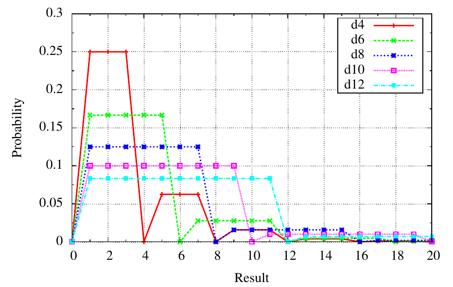
For 11 possible sums, listing the probabilities is manageable, albeit somewhat tedious. The same information is often displayed graphically. First, let's simply plot the probabilities in the table above.

Probability mass function (pmf) of 2d6

This plot shows the probability mass function (pmf) of the random variable given by the sum of rolling 2d6. On the plot we can see the probability increase linearly form 2 to 7, where it peaks, and then decrease from 7 to 12.

Wednesday, April 1, 2020

What's the probability of rolling doubles on 2d6?

I previously stated that the probability of rolling doubles on two six-sided dice is $1/6$.  Now I'll show why that's the case.

We can consider rolling one die first and then the other.  In order to roll doubles, we can get anything on the first die, but the second die must match it.  The probability of getting a specific result on the second die is $1/6$.  Thus, the probability of rolling double is $1/6$.  We can write this chain of thought as,
\begin{align}
P(\text{doubles on 2d6}) &= \sum_{x=1}^6 P(X_1 = x) \cdot P(X_2 = x) \\
&= \sum_{x=1}^6 P(X_1 = X_2 | X_2 = x) \cdot P(X_2 = x) \\
&= \sum_{x=1}^6 P(X_1 = X_2) \cdot P(X_2 = x) \\
&= P(X_1 = X_2) \cdot \sum_{x=1}^6 P(X_2 = x) \\
&= \frac{1}{6} \sum_{x=1}^6 \cdot P(X_2 = x) \\
&= \frac{1}{6} \cdot 6 \cdot \frac{1}{6} \\
&= \frac{1}{6}
\end{align}
where $X_1$ and $X_2$ are random variables representing the result of the first die and second die, respectively, and $x$ represents the value being matched.  In case you aren't familiar with the sigma notation, $\sum_{x=1}^6 f(x)$ is the sum of $f(x)$ over each integer value of $x$ starting at 1 and ending at 6 (note that sometimes the summation limits are written in slightly different places relative to the capital greek letter $\Sigma$).  Here $P(X_1 = X_2 | X_2 = x)$ is the probability that the two dice are equal conditioned on $X_2=x$.  Since the probability is independent of $x$ (for $x \in {1,2,3,4,5,6}$), the value is a constant $1/6$.

A derivation that is likely easier to grasp mathematically follows.
\begin{align}
P(\text{doubles on 2d6}) &= \sum_{x=1}^6 P(X_1 = x) \cdot P(X_2 = x) \\
&= \sum_{x=1}^6 \frac{1}{6} \cdot \frac{1}{6} \\
&= 6 \cdot \frac{1}{6} \cdot \frac{1}{6} \\
&= \frac{1}{6}
\end{align}
The probability of getting doubles is the sum of the probabilities of all specific cases of getting doubles.  Each specific case (e.g. rolling two ones) occurs with probability $\frac{1}{6}\cdot\frac{1}{6}$, since both dice must have that value.  There are a total of six cases, one for each possible value.

This generalizes to other types of dice simply.  Namely, for two $N$-sided dice (here I'm assuming these dice are numbered 1 through $N$), the probability of rolling doubles is $\frac{1}{N}$.  I'll leave showing this as an exercise for the reader (hint: replace every "6" above with "$N$").

But what about two dice of different types?  Suppose we have an $M$-sided die and an $N$-sided die (again, numbered 1–$M$ and 1–$N$, respectively — can I use respectively like this in parentheses?).  Similarly to before, this is the sum of the probabilities that $X_M$ and $X_N$ are equal for each possible value of $x$.
\begin{align}
P(\text{doubles on }1\text{d}M+1\text{d}N) &= P(X_M = X_N) \\
&= \sum_{x} P(X_M = x)\cdot P(X_N = x)
\end{align}
Since the probabilities $P(X_M = x)$ and $P(X_N = x)$ are only non-zero from 1–$M$ and 1–$N$, respectively, we only need to sum over the range $1 \leq x \leq \text{min}(M, N)$.  Without loss of generality, we may assume that $M < N$.  Thus,
\begin{align}
P(\text{doubles on }1\text{d}M+1\text{d}N)  &= \sum_{x=1}^M P(X_M = x)\cdot P(X_N = x) .
\end{align}
Over this range, we know that probabilities of getting any given value are $1/M$ and $1/N$, respectively.
\begin{align}
P(\text{doubles on }1\text{d}M+1\text{d}N)  &= \sum_{x=1}^M \frac{1}{M} \cdot \frac{1}{N} \\
&= M \cdot \frac{1}{M} \cdot \frac{1}{N} \\
&= \frac{1}{N}
\end{align}
This follows our earlier explanation.  No matter what we roll on the die with fewer sides, the probability of rolling the same on the second is 1 divided by the number of sides on the die with more sides.

We could envision rolling the die with more faces first, but the computation would be more involved, since the probability of matching given we roll a value not available on the die with fewer faces is zero.  The final result must, of course, match.

A Case for Theory

I've often seen a gamer post a question in an online forum like:
What's the probability of rolling doubles on 2d6?
Responses generally look like this:
16%
or this:
anydice.com
I find both responses deficient. The first simply gives an answer without teaching anything. (It is also incorrect. The probability is $1/6 = 0.1\overline{6}\approx17\%$. We'll calculate this later.)  If a second question arises, our gamer is back in the same situation as before. Also, if the question is related to a game design, if the answer isn't satisfactory, the designer has no knowledge to help change the design for the better. In fact, without a proper context and understanding of the mathematics, it may even be hard to know what questions need to be asked.

The second response seems somewhat better (although it may seem flippant or patronizing), as it gives our gamer a tool to answer not only this question, but any question of a similar nature. However, I think it's an even worse answer. Tools like anydice are fine as far as they go, but without a proper theoretical foundation they can be useless or even dangerous. While using the tool, apparent patterns will inevitably manifest. These may or may not be real since, as we hopefully all know, correlation is not causation.

The responses above are examples of generosity towards fellow gamers, for which we should be grateful. They offer a fish; my goal is to help to learn to fish. With a proper basis in the appropriate mathematical theory, a gamer should be able to
  • ask the right questions,
  • answer them independently,
  • know what the results mean, and
  • have some idea of what to do if the results aren't satisfactory.
Furthermore, experience and intuition should help to
  • make good assumptions and approximations and
  • determine the limitations of an analysis due to the assumptions made.
This blog discusses and applies a number of mathematical concepts and tools within the context of games. The games discussed are primarily tabletop games, including board games, card games, and roleplaying games.