Rolling ability scores in D&D

There are six main ability scores that have persisted through all editions of Dungeons & Dragons (although their order has changed). In the earlier editions, for each you would roll 3d6 to get a scores from 3–18, which may then be modified by various choices. Newer editions and house rules are often more generous to the player. This 3d6 method is often said to generate a "bell curve" of possible values, referring to the shape of the normal, or Gaussian, distribution's probability density function. I'll briefly get ahead of myself to point out the difference between the two shown in Fig. 1. They're pretty similar, but don't quite match. This comes from the central limit theorem, which tells that as we add up independent and identically distributed (i.i.d.) random variables the distribution of the sum converges to the normal distribution as the number of addends (i.e. the number of terms in the sum). approaches infinity. Each of the 3d6 that we roll are i.i.d, and even with only three terms we're already looking quite a bit like a bell curve, even though it's actually piece-wise quadratic. So the bell curve descriptor is not baseless, but it's not precise.

Figure 1: PMF of 3d6 compared to a bell curve

Let's go back and derive the pmf we just saw.

At first we might attempt to extend the method we used to compute the pmf of 1d$N$+1d$M$ in our discussion related to the dots in Catan. This works up to a point. We know there are $6^3= 216$ possible outcomes from rolling 3d6. For each sum we can count the number of ways to generate that sum with three numbers valued 1–6 by looking at the number of ways to put two separators on the inside of that many pips. For example, for a sum of 6, we can see that there are 5 choose 2, or $\binom{5}{2} = 5! / (3! \cdot 2!) = 10$ ways to do it. The 5 slots are illustrated below.

* | * | * | * | * | *

Unfortunately, this breaks down as we get to larger sums. For example, let's consider a sum of 9. We might think that there are 7 choose 2 possible combinations. However, some of those are invalid, like the one below.

* | * * * * * * * | *

Here we've chosen the separators such that the three dice sum to 9 with the values 1, 7, and 1. However, 7 is not a valid result on 1d6. We've over counted. We may be able to figure out how much we're over counting by and subtract that number out. However, it's going to be kludgey and probably not give us an equation from which we can glean anything intuitively. Thus, I'm not very interested in doing that. Let's find a better way.

To do that, I'll introduce the probability generating function (pgf). This is related to the moment generating function and the characteristic function of a random variable in ways that we won't get into here. The probability generating function $G_X(z)$ of a non-negative random variable $X$ with probability mass function $f_X(x)$ is defined as the expected value of $z^X$.
\begin{align}
G_X(z) &= \mathbb{E} z^X \\
&= \sum_{x=0}^\infty f_X(x) z^x
\end{align}
This looks very much like the $z$-transform of the probability mass function, the only exception being that we have a positive exponent of $z$, whereas the $z$-transform has a negative exponent. However, given that this function is only expected to converge for complex values of $z$ where $|z| \leq 1$, this difference is relatively minor. This gives us access to a bunch of tools and properties if we're familiar with the $z$-transform, which is related to Fourier and Laplace transforms, but for discrete-time signals. We won't get into all of them, but I'll show you the one we'll use here.

Let's say that $Y$ is the sum of rolling 3d6, where each die has its own result given by $X_1$, $X_2$, and $X_3$. The pmf of any of $X_1$, $X_2$, and $X_3$ is given as follows.
\begin{align}
f_X(x) &= \begin{cases}
\dfrac{1}{6} & \qquad x \in \{1, 2, 3, 4, 5, 6\} \\
0 &\qquad \text{else}
\end{cases}
\end{align}
Thus, the pgf is given by.
\begin{align}
G_X(z) &= \frac{1}{6} \left ( z^1 + z^2 + z^3 + z^4 + z^5 + z^6 \right )
\end{align}
Looking at the pgf of $Y$, we find an interesting property.
\begin{align}
G_Y(z) &= \mathbb{E} z^Y \\
&= \mathbb{E} z^{X_1+X_2+X_3} \\
&= \mathbb{E} z^{X_1} \cdot z^{X_2} \cdot z^{X_3} \\
&= \mathbb{E} z^{X_1}\mathbb{E}\cdot z^{X_2}\mathbb{E}\cdot z^{X_3} \\
&=G_{X_1}(z) \cdot G_{X_2}(z) \cdot G_{X_3}(z) \\
&= G_X(z)^3
\end{align}
When we sum random variables, the pgf of the sum is the product of the pgfs of the addends. Let's do this first for the 2d6 case, where $Y_2 = X_1 + X_2$.
\begin{align}
G_{Y_2}(z) &= G_X(z)^2 \\
&= \left( \frac{1}{6} \left ( z^1 + z^2 + z^3 + z^4 + z^5 + z^6 \right ) \right)^2 \\
&= \frac{1}{6^2} \left ( z^1 + z^2 + z^3 + z^4 + z^5 + z^6 \right ) ^2
\end{align}
Now let's multiply this out.
\begin{align*}
G_{Y_2}(z) = \frac{1}{6^2} ( z^2 +& z^3 + &z^4 +& z^5 +& z^6 +& z^7 + &&&&& \\
&z^3 + &z^4 + &z^5 + &z^6 + &z^7 + &z^8 +&&&&\\
&& z^4 + &z^5 + &z^6 + &z^7 + &z^8 + &z^9+&&&\\
&& &z^5 + &z^6 + &z^7 + &z^8 + &z^9 +&z^{10}+&&\\
&& & &z^6 + &z^7 + &z^8 + &z^9 +&z^{10} +&z^{11}+&\\
&&& & &z^7 + &z^8 + &z^9 +&z^{10}+&z^{11}+&z^{12} ) \hfill\\
\end{align*}
For our simple case, I think it's pretty clear that $f_{Y_2}(y)$ is the coefficient of the $z^y$ term. By grouping the like terms, which I've aligned vertically, we can see the familiar triangular shape of the 2d6 pmf.

A more computationally efficient way of looking at this is to take advantage of a property of $z$-transforms. Namely, that multiplication in the $z$ domain is convolution in the $x$ domain. (This is often stated as multiplication in the frequency domain is convolution in the time domain, although those are not the types of variables we're looking at. The opposite is also true: multiplication in the time domain is convolution in the frequency domain.) The convolution of two functions of integers, $f()$ and $h()$, is written as follows.
\begin{align}
f(x) * h(x) &= \sum_{n=-\infty}^\infty f(n) \cdot h(x-n)
\end{align}
Convolution is symmetric, so we can write either function first.
\begin{align}
f(x) * h(x) &= \sum_{n=-\infty}^\infty f(x-n) \cdot h(n) \\
&= h(x) * f(x)
\end{align}
Let's understand what this is doing graphically a little bit. The following figures depict various values of the convolution computation. The first plot in each figure shows one pmf function. The second plot shows the second pmf, which is flipped horizontally and shifted by the value at which the convolution is being computed. The third plot shows the multiplication of these two functions for each value of $n$. The fourth plot shows the result of the convolution, which at each value of $x$ is equal to the sum of the third plot across all $n$ for that value of $x$. As $x$ changes, it moves the flipped pmf horizontally. When it overlaps with the first pmf the result of the convolution is nonzero. When the two pmfs line up the convolution is maximized. Since the pmfs are either $1/6$ or 0, the product term takes on the value $1/36$ for some set of $n$. As the overlap increases, the result of the convolution increases linearly. Note that for $x=8$ the overlap starts decreasing, and so does the result of the convolution.

Figure 2: Illustrating convolution to find 2d6 pmf

We can repeat this process to find the pmf of 3d6 by convolving the previous result with the pmf of 1d6. In this case, the product term increases linearly once the overlap starts and continues through $x=8$. Up to the point, it's somewhat clear that the resulting pmf is given by,
\begin{align}
f_Y(y) &= \sum_{n=2}^{y-1} f_{Y_2}(n) .
\end{align}
Since $f_{Y_2}(n)$ is linear in that range, we can easily substitute it in.
\begin{align}
f_Y(y) &= \sum_{n=2}^{y-1} \frac{n-1}{6^2} \\
&= \sum_{n=1}^{y-2} \frac{n}{6^2}
\end{align}
You may recall that the sum of integers 1 to $n$ is equal to $n\cdot(n+1)/2$. If not, we can quickly prove this by induction. Consider $n=2$, the sum,
\begin{align}
\sum_{k=1}^2 k &= 1 + 2 = 3.
\end{align}
And when we evaluate $n\cdot(n+1)/2$ for $n=2$ we get $2 \cdot (2+1) / 2 = 3$. So it holds here. Now, let's assume it's true for $n$ and check if it holds for $n+1$.
\begin{align}
\sum_{k=1}^{n+1} k&= \left ( \sum_{k=1}^{n} k \right )+ (n+1) \\
&= \frac{n \cdot (n+1)}{2} + (n+1) \\
&=\frac{n \cdot (n+1) + 2\cdot(n+1)}{2} \\
&=\frac{(n+2) \cdot (n+1)}{2} \\
&=\frac{(n+1) \cdot (n+2)}{2}
\end{align}
We see that it does, thus it hold for all integer $n$. Multiplying this out we see clearly that this is a quadratic function.
\begin{align}
\sum_{k=1}^{n} k &= \frac{n \cdot (n+1)}{2} = \frac{1}{2}n^2 + \frac{1}{2} n
\end{align}
This holds for the other regions of this function as well. In general, if we calculate a running sum of a linear function, we'll get a quadratic function. If we do it piecewise, it holds piecewise. This extends to higher orders as well, as expressed in Faulhaber's formula.

Below we see the same plots showing how $f_Y(y)$ is calculated using the following convolution.
\begin{align}
f_Y(y) = f_{Y_2}(y) * f_X(y)
\end{align}

Figure 3: Illustrating convolution to find 3d6 pmf

This solution appears unsatisfying in some ways. We have a result we can express in an equation, but we can't look at it directly and glean much information. However, what we often care about are having an intuitive understanding of what the result is and an easy way to calculate it numerically. We do have both of those. The central limit theorem and the properties of convolution we looked at here gives us the intuitive understanding. We can also extend this by looking at specific critical values, such as the extreme and central values. Calculating it is also simple. Many tools have simple functions to compute this convolution, so that we can easily tabulate or plot any specific case that we're interested in.

Should I draw a face-up wild in Ticket to Ride?

The inevitably unsatisfying short answer is: it depends. (Of course, if a game offers a choice, but one option is always best, then it's not really a choice, but it's still taking up rules complexity.) Let me set up the condition I'm thinking about. It's your turn, you don't want to build, draw more tickets, or run a passenger (I have the Märklin edition), so you're going to draw cards. None of the face-up cards interest you except possibly a locomotive. So should you draw the face-up wild or top deck?

One account could look at the expected value of the number of useful cards you'll get on this turn. Drawing the face-up wild it's clear that you'll always get one useful card (assuming you're still going to build something). But what if you draw off the top? You might get something good, you might not. Moreover, since you'll draw two cards there's even a middling outcome. For simplicity, let's consider cards to be either useful or useless for you. Thus, you could end up better or worse than drawing the face-up wild. The probability of each case depending on how many cards are useful to you. We'll assume that $c$ colors are useful to you. For simplicity, let's also assume that at least two cards of any useful color are useful. We've certainly put a lot of caveats and assumptions in, which is often necessary to get a first clean result.

Now let's look at the composition of the deck. In Ticket to Ride there are 110 cards: 12 of each of 8 colors plus 14 locomotives (wilds). (Most versions have this deck composition, but the Märklin edition is different.) In reality, you'll know a lot of information about cards in your hand, other cards available to draw, cards in the discard pile, maybe even some you remember that are in other players' hands. However, we're going to look at the general case where almost none of that is taken into account. This averages our result across all possibilities. Given the fact that the deck has over 100 cards and we're drawing only two, these effects don't often have large impacts. The number of useful cards, $n$, is 14 cards, which are always useful (wilds), plus 12 for each useful suit.
\begin{align}
n = 12 \cdot c + 14
\end{align}
We can simplify the answer by approximating the probabilities of the card draws as independent. Thus, for each of the two cards drawn, the probability that it's useful is approximately,
\begin{align}
P(\text{useful}) &= \frac{n}{110} \\
&= \frac{12\cdot c + 14}{110}
\end{align}
Let's consider the scale of the error some of our assumptions and approximations are introducing. We're ignoring the five cards face up and the first card drawn when considering the second. Thus, the true probability can fall within the following range.
\begin{align}
\frac{n-6}{110-6} \leq p \leq \frac{n+6}{110-6}
\end{align}
That's actually a bit loose. We just tacitly assumed that these six cards could be either useful or not. However, we know that's not true. Specifically, we know that of the face-up cards, the only useful ones are wild cards, of which there can be at most two (given the rules about clearing the display for three). Given the choice we're making, we know there's at least one face-up wild card. Taking this into account, we can update our approximate probability assuming one face-up wild card. We know five of the 110 cards, and that one of them is useful.
\begin{align}
P(\text{useful}) &= \frac{n-1}{110-5} \\
&= \frac{12\cdot c + 13}{105}
\end{align}
Note that we're not assuming that 105 cards are in the draw pile. Instead, we're saying that we don't know anything about where any of them are. If some are in the discard pile and some are in other players' hand, but we don't know what cards they are, the probability is the same. Taking this into account, we can see the approximation error from assuming that the card draw probabilities are independent is small. The probability of the second card given the first would be one of the following two.
\begin{align}
P(\text{second useful} | \text{first useful}) &= \frac{12\cdot c + 13 -1 }{105 -1} \\
&= \frac{12 \cdot c + 12}{104} \\
P(\text{second useful} | \text{first useless}) &= \frac{12\cdot c + 13 + 1 }{105 -1} \\
&= \frac{12 \cdot c + 14}{104}
\end{align}
From we these we can find the approximation errors.
\begin{align}
\epsilon_1 &= P(\text{useful}) - P(\text{second useful} | \text{first useful}) \\
&= \frac{12\cdot c + 13}{105} - \frac{12 \cdot c + 12}{104} \\
&= \frac{ 104 \cdot (12 c + 13) - 105 \cdot (12c + 12)}{104 \cdot 104} \\
&= \frac{ -12 c + 92}{10920} \\
&= \frac{ -3 c + 23}{2730} \\
&\approx -0.0011c + 0.0084
\end{align}
Since the number of useful colors can range from 1 to 7, this first error can range from about 0.0007 to 0.0073, less than 1% in either case. Similarly for the other case.
\begin{align}
\epsilon_2 &= P(\text{useful}) - P(\text{second useful} | \text{first useless}) \\
&= \frac{12\cdot c + 13}{105} - \frac{12 \cdot c + 13}{104} \\
&= \frac{ 104 \cdot (12 c + 13) - 105 \cdot (12c + 13)}{104 \cdot 104} \\
&= \frac{ -12 c -13}{10920} \\
&\approx -0.0023c - 0.0012
\end{align}
Here the error can be somewhat larger in magnitude, ranging from $-0.012$ to $-0.0089$, but still less than 1%.

I go through this exercise to make clear that we can make simplifications like this. I've probably used more words justifying it than I would have taking the full probabilities into consideration. To quickly check or bound the error for yourself is much faster.

Knowing the probability that each draw is useful, we can look at the distribution of the number of useful cards when drawing from the top here. This is another binomial distribution, although with two draws it's pretty transparent. If the number of useful cards we draw is the random variable $U$, then we can express the probabilities as follows.
\begin{align}
P(U = 0) & = \left ( 1 - P(\text{useful}) \right ) ^2 \\
&= \left ( 1 - \frac{12 \cdot c + 13}{105} \right ) ^2 \\
&= \left ( \frac{104 - (12c + 13)}{105} \right ) ^2 \\
&= \left ( \frac{92 - 12c}{105} \right ) ^2 \\
P(U = 1) & = 2 \cdot P(\text{useful}) \cdot \left ( 1 - P(\text{useful}) \right ) \\
&= 2 \cdot \frac{12 \cdot c + 13}{105} \cdot \left ( 1 - \frac{12 \cdot c + 13}{105} \right ) \\
&= 2 \cdot \frac{12 \cdot c + 13}{105} \cdot \frac{92 - 12c}{105} \\
P(U = 2) &= P(\text{useful}) ^2 \\
& = \left ( \frac{12 \cdot c + 13}{105} \right ) ^2

\end{align}
Each of these are plotted as a function of the number of useful colors in Fig. 1. As there are three possibilities, it's not necessarily clear what we should make of this. All three probabilities are second-order functions of $c$, which we can see in their parabolic shape. Two alternative ways are the probability of getting one or more useful card and the expected value of the number of useful cards, respectively.

Figure 1: Probabilities when top-decking in Ticket to Ride

The probability of getting one or more card is the sum of the probabilities of getting one and two cards.
\begin{align}
P(U \geq 1) &= P(U = 1) + P(U = 2) \\
&= 2 \cdot \frac{12 \cdot c + 13}{105} \cdot \frac{92 - 12c}{105} + \left ( \frac{12 \cdot c + 13}{105} \right ) ^2 \\
&= 2\cdot \frac{-144c^2+948c +1196}{105^2} + \frac{144c^2+312c+169}{105^2} \\
&= \frac{-288c^2+1896c +2392 + 144c^2+312c+169}{105^2} \\
&= \frac{-144c^2+2208c +2561}{105^2}

\end{align}
This function is also plotted in Fig. 1. This indicates that when two or more colors are useful, you're more likely than not to get at least one useful card. On the other hand, it's still quite likely that you'll get nothing useful.

Figure 2: Expected useful cards when top-decking in Ticket to Ride

Recall the expected value is the weighted average of a random variable, and given here by,
\begin{align}
\mathbb{E} U = \sum_u u \cdot P(U=u).
\end{align}
This ends up being the sum of just the two possible non-zero terms.
\begin{align}
\mathbb{E} U &= 1 \cdot P(U = 1) + 2 \cdot P(U = 2) \\
&=2 \cdot \frac{12 \cdot c + 13}{105} \cdot \frac{92 - 12c}{105} + 2 \cdot \left ( \frac{12 \cdot c + 13}{105} \right ) ^2 \\
&= 2\cdot \frac{-144c^2+948c +1196}{105^2} + 2\cdot\frac{144c^2+312c+169}{105^2} \\
&=2\cdot\frac{1260c+1365}{105^2} \\
&=2\cdot\frac{12c+13}{105}
\end{align}
Alternatively, we can do the algebra at a higher level of abstraction, where we're less prone to arithmetic mistakes.
\begin{align}
&= 2 \cdot P(\text{useful}) \cdot \left ( 1 - P(\text{useful}) \right ) + 2 \cdot P(\text{useful}) ^2 \\
&= 2 \cdot P(\text{useful}) - \require{cancel}\cancel{2 \cdot P(\text{useful}) \cdot P(\text{useful})} + \cancel{2 \cdot P(\text{useful})^2} \\
&= 2 \cdot \frac{12 \cdot c + 13}{105}\\
&= \frac{24 \cdot c + 26}{105}\\
&\approx 0.23 c + 0.25

\end{align}
We see that the quadratic terms canceled out and we're left with a linear equation, as shown in Fig. 2. This makes sense. Given that we approximated the two draws as independent, the expected value of the number of useful cards when drawing two cards should be twice that as when drawing one card. Expectation is linear. The expected value for a single draw, $U_1$, should be proportional to the number of useful cards available in the deck.
\begin{align}
\mathbb{E} U_1 &= 0 \cdot P(U_1 = 0) + 1 \cdot P(U_1 = 1) \\
&= P(U_1 = 1) \\
&= P(\text{useful}) \\
&= \frac{12\cdot c + 13}{105} \\
 &\approx 0.11 c + 0.12
\end{align}
According to the plot, when four or more colors are useful we expect to get more than one useful card. Looking at the earlier result, we see that there's still a pretty substantial chance that you'll get nothing useful, $P(\text{0 useful cards} | c = 4) \approx 0.2$. Which is the correct way to think about it? They're both useful. The expected value essentially tells you what you'd get on average if you repeated this an infinite number of times. This is known from the strong law of large number, which states that the sample average converges almost surely to the mean as the sample size goes to infinity. Here almost surely has the specific meaning that it occurs with probability 1. Note that this is distinct from always happening and is perhaps best understood with continuous-valued random variables which tend not to come up for us here. A nice property is that it takes into account the benefit of sometimes getting two useful cards. So as a general strategy, it makes sense to look at the expected value.

However, using the expected value breaks down in two ways here. First, it violates the approximating assumption that the card draws are independent. That's a reasonable approximation for two cards, but becomes less so as more cards are drawn. So our approximate expected value is really only the average of a single draw across many separate games. Second, the number of times that this comes up in a game isn't that large. For many values of $c$, the probabilities of getting either no useful cards and two useful cards are both substantial. Thus, you'd expect to see scenarios where you come up empty-handed and others where you do much better drawing from the top. On the other hand, drawing the wild card is more reliable. It's the low variance play.

How far can I throw in a tunnel?

As pointed out in this video from LindyBeige, if you are inside, say, a dungeon, then low ceilings limit how far you can throw javelins and the like because they rely on you throwing them high to achieve distance. So the question is, if you know the ceiling height, how far can you throw?

Let's assume that we know how far you can throw outside, where you're not limited by ceilings. This aligns with the maximum range that may be listed in a game's rules. For example, in Dungeons and Dragons, a javelin has a long range of 120'. For simplicity, let's assume the ceiling is uniform is height. (Yes, this directly contradicts the first point in LindyBeige's video.)

When you throw, you can choose the angle at which you throw. Inside, you'll use a lower angle to avoid the ceiling. But let's assume that you throw with the same initial speed. Gravity pulls the javelin down and air pushes against the direction of movement. We'll account for the first, but ignore the second. Ignoring air resistance is par for the course when doing analyses such as this, often without regard for whether or not it's appropriate. Our first task is to deduce the initial speed based on the outside throwing range. Let $x_f$ be this range. We'll break up the initial velocity into its horizontal component, $v_{x0}$, and its vertical component, $v_{y0}$. Gravity provides a constant acceleration, the rate of change in velocity, so we know the velocity as a function of time and the gravitational constant $g = 9.8 \, \text{m}/\text{s}$.
\begin{align}
v_y(t) = v_{y0} -  g\cdot t
\end{align}
From this we can determine the elevation of the javelin throughout its flight, $y(t)$. Here we'll reference zero height at the normal height of a person, assuming that since the target is about equal in height to the launch height, so $y(0) = y_0 = 0$. The change in height is determined by integrating the velocity.
\begin{align}
y(t) &= y_0 + \int_0^t v(t) \,\mathrm{d}t \\
y(t) &= \int_0^t  v_{y0} -  g\cdot t  \,\mathrm{d}t \\
y(t) &=  v_{y0} \cdot t -  \frac{1}{2} \cdot g\cdot t^2
\end{align}
Using this we can solve for the time at which the javelin reaches the target height of $y(t) = 0$, which occurs at the final time $t_f$.
\begin{align}
y(t_f) &= 0 \\
0 &= v_{y0} \cdot t_f -  \frac{1}{2} \cdot g\cdot t_f^2  \\
\end{align}
We're interested in the case when $y(t) = 0$ but $t \neq 0$, so we can divide by $t_f$ and then solve for it.
\begin{align}
0 &= v_{y0} -  \frac{1}{2} \cdot g\cdot t_f  \\
\frac{1}{2} \cdot g\cdot t_f & =v_{y0} \\
t_f &= \frac{v_{y0}}{\frac{1}{2} \cdot g} \\
t_f &= 2 \cdot \frac{v_{y0}}{g}
\end{align}
This tells us how much time the javelin spends in the air. Next, we can find how far it travels based on this. Since you're not throwing it straight up, there's some initial horizontal component to the velocity, $v_{x0}$. We'll specify the horizontal position, $x$, to have value $0$ at $t=0$ where you throw from, so the horizontal position is simply proportional to time and initial horizontal velocity. In fact, this position is equal to the product of these two.
\begin{align}
x(t) = v_{x0} \cdot t
\end{align}
Thus the distance thrown, $x_f = x(t_f)$ is as follows.
\begin{align}
x_f &= v_{x0} \cdot t_f \\
&= v_{x0} \cdot 2 \cdot \frac{v_{y0}}{g} \\
&=  \frac{2 \cdot v_{x0} \cdot v_{y0}}{g}
\end{align}
Next, we can find the optimal way to split the initial velocity $v_0$ between its vertical and horizontal components. The initial velocity is a vector, having both magnitude, $|v_0|$ and an angle $\angle v_0$. We can use trigonometric functions to relate the initial velocity into its Cartesian components.
\begin{align}
v_{x0} &= |v_0| \cos  \angle v_0  \\
v_{y0} &= |v_0| \sin  \angle v_0
\end{align}
We don't ultimately care about the angle, so we can also just look at the magnitude, using the Pythagorean formula.
\begin{align}
|v_0|^2 &= v_{x0}^2 + v_{y0}^2
\end{align}
From this we can solve for $v_{x0}$.
\begin{align}
v_{y0} &=  \sqrt{|v_0|^2 - v_{x0}^2}
\end{align}
We can use this to go back and find the distance thrown in terms of $v_0$ and $v_{y0}$.
\begin{align}
x_f &=   \frac{2  \cdot v_{x0} \cdot \sqrt{|v_0|^2 - v_{x0}^2}}{g}
\end{align}
The final distance reached is a function of the initial horizontal velocity component. We anticipate a maximum, so let's take the derivative of the final position with respect to this velocity component and find where it's zero.
\begin{align}
0 & = \frac{ \mathrm{d} x_f } {  \mathrm{d} v_{x0}  } \\
0 &= \frac{ \mathrm{d} } {  \mathrm{d} v_{x0}  }   \frac{2  \cdot v_{x0} \cdot \sqrt{|v_0|^2 - v_{x0}^2}}{g}  \\
0 &=  \frac{2 }{g} \cdot \frac{ \mathrm{d} } {  \mathrm{d} v_{x0}  }   \cdot v_{x0} \cdot \sqrt{|v_0|^2 - v_{x0}^2}  \\
0 &=  \frac{2 }{g} \cdot \left ( \sqrt{|v_0|^2 - v_{x0}^2} + v_{x0} \cdot \frac{1}{2} { \left (|v_0|^2 - v_{x0}^2 \right )}^{-\frac{1}{2}}\cdot  \frac{ \mathrm{d} } {  \mathrm{d} v_{x0}  } |v_0|^2 - v_{x0}^2 \right ) \\
0 &=  \frac{2 }{g} \cdot \left ( \sqrt{|v_0|^2 - v_{x0}^2} + v_{x0} \cdot \require{cancel}\cancel{ \frac{1}{2}} { \left (|v_0|^2 - v_{x0}^2 \right )}^{-\frac{1}{2}}\cdot  -\cancel{2}\cdot v_{x0} \right ) \\
0 &=  \frac{2 }{g} \cdot \left ( \sqrt{|v_0|^2 - v_{x0}^2} -  v_{x0} \cdot { \left (|v_0|^2 - v_{x0}^2 \right )}^{-\frac{1}{2}}\cdot  v_{x0} \right ) \\
0 &=  \left ( \sqrt{|v_0|^2 - v_{x0}^2} -  \frac{v_{x0}^2}{\sqrt{|v_0|^2 - v_{x0}^2 }} \right ) \\
\end{align}
Now let's bring some stuff to both sides and rearrange.
\begin{align}
\frac{v_{x0}^2}{\sqrt{|v_0|^2 - v_{x0}^2 }} &=   \sqrt{|v_0|^2 - v_{x0}^2}  \\
\frac{v_{x0}^2}{\sqrt{|v_0|^2 - v_{x0}^2 }} \cdot  \sqrt{|v_0|^2 - v_{x0}^2}  &=   \sqrt{|v_0|^2 - v_{x0}^2} \cdot  \sqrt{|v_0|^2 - v_{x0}^2} \\
v_{x0}^2 & = |v_0|^2 - v_{x0}^2 \\
2 v_{x0}^2 & = |v_0|^2 \\
v_{x0}^2 & = \frac{1}{2} |v_0|^2
\end{align}
There's a solution to this where $v_{x0}$ and $|v_0|$ are both $0$, but we're not interested in that case.
\begin{align}
v_{x0} &= \frac{ |v_0| }{\sqrt{2}}
\end{align}
This is a simple case that we can recognize that $v_{y0}=1/ \sqrt{2} \cdot |v_0|$ also and $\angle v_0 = 45^\circ$. We can now plug this back into our previous equation to find a relationship between $x_f$ and $v_0$.
\begin{align}
x_f &=  \frac{2  \cdot  \frac{ |v_0| }{\sqrt{2}} \cdot \sqrt{|v_0|^2 -\left(  \frac{ |v_0| }{\sqrt{2}} \right )^2}}{g}  \\
&=  \frac{2  \cdot  \frac{ |v_0| }{\sqrt{2}} \cdot \sqrt{\frac{|v_0|^2}{2}}}{g}  \\
&=  \frac{2  \cdot  \frac{ |v_0| }{\sqrt{2}} \cdot \frac{ |v_0| }{\sqrt{2}}}{g}  \\
&=  \frac{\require{cancel}\cancel{2}  \cdot  \frac{|v_0|^2}{\cancel{2}} }{g}  \\
x_f &=  \frac{|v_0|^2}{g}  \\
|v_0|^2 &= g \cdot x_f\\
|v_0| &= \sqrt{g \cdot x_f}
\end{align}
All this work has been done to give us the initial speed as a function of the distance thrown outside. Now we can turn our attention to how far we can throw given this initial velocity and a ceiling height. Let's set the maximum height of the javelin in flight to be $y_p$, where our $p$ is for peak. We'll say that this occurs at time $t_p$.
\begin{align}
y_p &= y(t_p)
\end{align}
To try to keep our variables from getting confused, we'll specify different vertical and horizontal components to the velocity now that you're throwing inside. Let these be $v_{yi}$ and $v_{xi}$, respectively.
\begin{align}
y_p &= v_{yi} \cdot t_p -  \frac{1}{2} \cdot g\cdot t_p^2
\end{align}
We'll find where the derivative is zero again to find the time at which the maximum height occurs maximum again.
\begin{align}
0 &= \frac{ \mathrm{d} y(t) } {  \mathrm{d} t  } \\
0 &= \frac{ \mathrm{d} } {  \mathrm{d} t  }  \left ( v_{yi} \cdot t -  \frac{1}{2} \cdot g\cdot t^2 \right )\\
0 &=    v_{yi}  -    g\cdot t\\
g\cdot t &=  v_{yi}   \\
t &= \frac{v_{yi}}{g}\\
t_p &= \frac{v_{yi}}{g}
\end{align}
Now we can find the maximum height by plugging in this time.
\begin{align}
y_p &= v_{yi} \cdot \frac{v_{yi}}{g} -  \frac{1}{2} \cdot g\cdot \left ( \frac{v_{yi}}{g} \right ) ^2 \\
&= \frac{v_{yi}^2}{g} -  \frac{1}{2} \cdot g\cdot  \frac{v_{yi}^2}{g^2}  \\
&= \frac{v_{yi}^2}{g} -  \frac{1}{2} \cdot   \frac{v_{yi}^2}{g}  \\
y_p &=   \frac{1}{2} \cdot  \frac{v_{yi}^2}{g}   \\
v_{yi}^2 &= 2 \cdot g \cdot y_p \\
v_{yi} &= \sqrt{2 \cdot g \cdot y_p }
\end{align}
Based on the previous equation for the final distance, we can find the write the final inside distance, $x_{fi}$, in terms of the initial velocity components.
\begin{align}
&=  \frac{2 \cdot v_{xi} \cdot v_{yi}}{g} \\
&=  \frac{2 \cdot \sqrt{|v_0|^2 - v_{yi}^2} \cdot v_{yi}}{g}  \\
&=  \frac{2 \cdot \sqrt{|v_0|^2 - 2 \cdot g \cdot y_p } \cdot \sqrt{2 \cdot g \cdot y_p }}{g}  \\
&=  \frac{2 \cdot \sqrt{\left (  \sqrt{g \cdot x_f} \right)^2 - 2 \cdot g \cdot y_p } \cdot \sqrt{2 \cdot g \cdot y_p }}{g}  \\
&=  \frac{2 \cdot \sqrt{\require{cancel}\cancel{g} \cdot x_f- 2 \cdot \cancel{g} \cdot y_p } \cdot \sqrt{2 \cdot \cancel{ g} \cdot y_p }}{\cancel{g}}  \\
x_{fi} &=  2 \cdot \sqrt{x_f - 2  \cdot y_p } \cdot \sqrt{2  \cdot y_p }
\end{align}
Note that this only applies when $y_p$ is less than the maximum height outside. As an example with the javelin's range of 120 ft in a 10 ft room, the maximum thrown distance in ft becomes,
\begin{align}
2 \cdot \sqrt{120 - 2  \cdot 10 } \cdot \sqrt{2  \cdot 10 }  \approx 89.4 .
\end{align}
There's a little gotcha here. We assumed zero elevation at the height of the thrower. Let's just call this 5 ft for simplicity. Thus, we should take 5 ft off the height that we plug into the equation above.
\begin{align}
2 \cdot \sqrt{120 - 2  \cdot (10-5) } \cdot \sqrt{2  \cdot (10-5) }  \approx 66.3
\end{align}

Another thing we need to take care of is the range over which our equation is valid. Now, since we're dealing with real numbers in the real world, we know that we must meet the condition $x_f > 2 \cdot y_p$, as otherwise we'd have a negative number inside the square root. However, we need to consider the case when the outdoor maximum height, $y_{max}$, is less than or equal to the elevation of the ceiling, $y_p$. To check, we'll go back and find $y_{max}$. If $y_p \geq y_{max}$ then the indoor range is equal to the outdoor range. To do this, let's recall some earlier equations.
\begin{align}
|v_0| &= \sqrt{g \cdot x_f} \\
v_{y0} &= \sqrt{2 \cdot g \cdot y_{max} } \\
v_{y0}&=\frac{1}{ \sqrt{2}} \cdot |v_0|
\end{align}
We can combine these and do some algebra to find the outdoor maximum height reached by the javelin.
\begin{align}
\sqrt{2 \cdot  g \cdot y_{max} } & = \frac{1}{ \sqrt{2}} \cdot |v_0| \\
2 \cdot g \cdot y_{max}  & = \frac{1}{2} \cdot |v_0|^2 \\
y_{max}  & = \frac{1}{4g} \cdot |v_0|^2 \\
y_{max}  & = \frac{1}{4g} \cdot \left (  \sqrt{g \cdot x_f} \right )^2 \\
y_{max}  & =  \frac{ x_f}{4}
\end{align}
So this means the maximum range is 4 times the height reached during flight outside. Thus, if the ceiling is at least one quarter of the outdoor range, it has no impact. To check that the points coincide, we can evaluate our equation for the indoor range when the ceiling is equal to $y_{max} = \frac{x_f}{4}$.
\begin{align}
x_{fi} &=  2 \cdot \sqrt{x_f - 2  \cdot \frac{x_f}{4} } \cdot \sqrt{2 \cdot \frac{x_f}{4} }  \\
& =  2 \cdot \sqrt{x_f - \frac{x_f}{2} } \cdot \sqrt{ \frac{x_f}{2} }  \\
& =  2 \cdot \sqrt{ \frac{x_f}{2} } \cdot \sqrt{ \frac{x_f}{2} }  \\
& =  2 \cdot \frac{x_f}{2} \\
& =  x_f
\end{align}
Indeed they match.

Putting this together we can get in the following equation.
\begin{align}
x_{fi} &= \begin{cases}
2 \cdot \sqrt{x_f - 2  \cdot y_p } \cdot \sqrt{2  \cdot y_p } & \text{if } y_p < \frac{x_f}{4} \\
x_f & \text{otherwise}
\end{cases}
\end{align}
This is shown below as plots of indoor range vs. outdoor range by ceiling height, assuming a 5' tall thrower. Some example indoor ranges, rounded to the nearest 5', for an assortment of outdoor ranges and ceiling heights are listed in the table at the end.

Indoor range by ceiling height

\begin{align}
\begin{array}{c|c|c|c|c|c|c|c}
\text{Ceiling Height}&  15& 60& 100& 120& 320& 400& 600 \\ \hline
 5&   0&    0&    0&    0&    0&    0&    0\\
10&  15&   45&   60&   65&  110&  125&  155\\
15&  15&   55&   80&   90&  155&  175&  215\\
20&  15&   60&   90&  105&  185&  210&  260\\
25&  15&   60&  100&  115&  210&  240&  300\\
30&  15&   60&  100&  120&  230&  265&  330\\
35&  15&   60&  100&  120&  250&  285&  360\\
40&  15&   60&  100&  120&  265&  305&  385\\
45&  15&   60&  100&  120&  275&  320&  410\\
50&  15&   60&  100&  120&  290&  335&  430\\
\end{array}\\
\text{Indoor ranges by outdoor ranges for project weapons, rounded to 5'}\\
\end{align}

What's the toughest unit in Memoir '44?

Note: there's some errata for this post here.

In Memoir '44, there are three primary units: Infantry, Armor, and Artillery. When you make an normal attack against a unit, you roll a number of dice based on the attacking circumstances (unit, range, etc) and remove one figure from the target for each symbol that either matches the target or is a grenade. The dice are six-sided dice with the following sides: 2 infantry, 1 armor, 1 flag, 1 star, and 1 grenade. Rolling a flag makes the target retreat, but we'll set this aspect aside for now. The infantry are the easiest to damage, as three of the six sides removes a figure. Armor have a $2/6$ chance of losing a figure for each attack die, while Artillery have only a $1/6$ chance of losing a figure because only a grenade does the job.

On the other hand, each of these units start with a different number of figures based on the type: Infantry have 4, Armor 3, and Artillery 2. This means that while Artillery are the hardest to hit, you need fewest hits to eliminate each one. Let's evaluate which of these effects win out. To do this, we'll determine how many dice it may take to eliminate each unit type.

It's tempting to think that we should look at the binomial distribution of the number of hits for different numbers of dice rolled. However, that would give us the probability that we get enough hits to eliminate a unit given that we roll a certain number of dice. For a small number of dice, which may be rolled in a single attack, that is correct, but for larger numbers, where dice are rolled across multiple attacks, it is wrong for the simple reason that can't attack a unit that's already eliminated. The probability of getting 4 hits when rolling 10 dice includes cases when the first 4 dice all get hits, so we'd never roll the subsequent 6 six. Another way of thinking about it, is that the binomial distribution could tell us what the probability is of eliminating a unit with up to a certain number of dice.

Instead, we'll consider rolling 1 attack die at a time. This sounds like the opposite extreme, but it applies directly to some cases and represents rolling multiple dice in each attack as well as we can, considering extra hits go unused. Right away we see some difference. For example, we can eliminate an Artillery unit with just 2 attack dice with a probability of $(\frac{1}{6})^2\approx 0.0278$, while the probability for Armor and Artillery is zero, since they have more than 2 figures each.

Let's assign some variables. Let's say the number of starting figures of a unit is $f$, the number of dice rolled to eliminate the target unit is a random variable $N$, and the probability of each die hitting is $p$. We'll use subscripts to denote the units. To eliminate a unit on the $n$-th roll, the $n$-th roll must be a hit and there must be exactly $f-1$ hits accumulated on previous rolls, for $f$ total hits. Since the number of hits and misses must sum to $n$, the number of misses is $n  - f$. Here, we'll leverage the binomial distribution to find the probability of getting $f-1$ hits in $n-1$ rolls, which has the probability mass function (pmf) $f_\text{binomial}(f-1; n-1,p)$. We can thus assemble the pmf of $N$, $f_N(n) = P(N= n)$, as follows.
\begin{align}
f_N(n) &= f_\text{binomial}(f-1; n-1, p) \cdot p \\
&= \binom{n-1}{f-1} \cdot  p^{f-1} \cdot (1-p)^{(n-1)-(f-1)} \cdot p \\
&= \binom{n-1}{f-1} \cdot  p^f \cdot (1-p)^{n-f}
\end{align}
Plugging in the binomial coefficient $n-1$ choose $f-1$, $\binom{n-1}{f-1}$, we find the following. Note that we should pay attention to the range of $n$ over which this is value. When $n < f$, we haven't rolled enough dice to to be able to eliminate the target unit. Earlier, with the binomial coefficient, this was somewhat implied, as we cannot, for example, choose 4 dice out of 3.
\begin{align}
f_N(n) &= \frac{(n-1)!}{(f-1)! ((n-1)-(f-1))!} \cdot  p^f \cdot (1-p)^{n-f} && f \leq n \\
&= \frac{(n-1)!}{(f-1)! (n-f)!} \cdot  p^f \cdot (1-p)^{n-f} && f \leq n \\
\end{align}
Here we've computed the pmf of the number of dice it takes to eliminate a unit, which I've plotted in Fig. 1. This naturally starts at 0 for $n < f$ and approaches 0 again for high $n$. This is because the sum over all $n$ must be 1, as the sum of the probabilities of all possibilities is 1. For each higher $n$, it's more and more likely that you would have eliminated the target in less than $n$ rolls.

Fig. 1: Memoir '44 probability of unit elimination

One striking feature of the plot is that for every unit type, the probability of elimination peaks at 6 and 7 dice, which appear to have equal probabilities. To check this, we can look at the difference equation for $f_N(n)$, which is similar to taking a derivative, but for functions of discrete-valued variables. Sometimes we might get away with using a derivative as a shortcut, however, the binomial coefficient here will get in our way. So what we want to look at is the difference of $f_N(n+1)$ and $f_N(n)$.
\begin{multline}
f_N(n+1) - f_N(n) = \frac{(n+1-1)!}{(f-1)! (n+1-f)!} \cdot  p^f \cdot (1-p)^{n+1-f} \\- \frac{(n-1)!}{(f-1)! (n-f)!} \cdot  p^f \cdot (1-p)^{n-f} \\
\end{multline}
Here, it's perhaps easier if we can write $f_N(n+1)$ in terms of $f_N(n)$, in order to express the difference more clearly.
\begin{align}
f_N(n+1) &= \frac{(n+1-1)!}{(f-1)! (n+1-f)!} \cdot  p^f \cdot (1-p)^{n+1-f} \\
&= \frac{n}{n+1-f} \cdot p \cdot \frac{(n-1)!}{(f-1)! (n-f)!} \cdot  p^f \cdot (1-p)^{n-f} \\
&= \frac{n}{n+1-f} \cdot (1- p) \cdot f_N(n)
\end{align}
Which gives us the difference as,
\begin{align}
f_N(n+1) - f_N(n) &= \left ( \frac{n \cdot (1- p)}{n+1-f} - 1 \right) \cdot f_N(n). \\
\end{align}
Or more explicitly,
\begin{multline}
f_N(n+1) - f_N(n) \\= \left ( \frac{n \cdot (1- p)}{n+1-f} - 1 \right) \cdot  \frac{(n-1)!}{(f-1)! (n-f)!} \cdot  p^f \cdot (1-p)^{n-f} .
\end{multline}
Now, $f_N(n)$ is non-negative, as it is a probability. That is $f_N(n) \geq 0$. Thus, any sign change in the difference must come from the first term, $ \left ( \frac{n \cdot (1- p)}{n+1-f} - 1 \right)$. Let's solve for when this is zero to look for the maxima that we observe.
\begin{align}
0 &= \left ( \frac{n \cdot (1- p)}{n+1-f} - 1 \right) \\
1 &= \frac{n \cdot (1- p)}{n+1-f} \\
n+1-f & = n \cdot (1- p) \\
\require{cancel}\cancel{n}+1-f & = \cancel{n} - n\cdot  p \\
1-f & = - n\cdot  p \\
n\cdot  p &= f - 1\\
n & = \frac{f-1}{p}
\end{align}
Now, note that we do have an interesting relationship between $f$ and $p$ for all three units.
\begin{align}
f_\text{infantry} &= 4 & p_\text{infantry}  &= \frac{3}{6} \\
f_\text{armor} &= 3 & p_\text{armor}  &= \frac{2}{6} \\
f_\text{artillery} &= 2 & p_\text{artillery} &= \frac{1}{6} \\
\end{align}
In each case we have the following relation.
\begin{align}
p = \frac{f-1}{6}
\end{align}
Plugging this into our equation for when the difference $f_N(n+1) - f_N(n) = 0$, we find that the difference is indeed zero.
\begin{align}
n & = \frac{f-1}{p}\\
& = \frac{\require{cancel}\cancel{f-1}}{\left (\cfrac{\cancel{f-1}}{6} \right )} \\
n& = 6
\end{align}
Thus, the probability of eliminating a unit when rolling the 6th die is the same as when rolling the 7th die, for all these unit types. If we had a unit that started with 5 figures and were hit with probability $4/6$, it would also have this property.

Looking at just the pmf doesn't give us a clear picture of which is best. The distribution for artillery is shorter and fatter than infantry. Another comparison we can make is to look at the probability that a unit is eliminated by the $n$-th die, that is, with $n$ or fewer dice.
\begin{align}
F_N(n) = \sum_{k=0}^{n} f_N(k)
\end{align}
This is the cumulative distribution function (CDF), which is plotted in Fig. 2.

Fig. 2: Memoir '44 cumulative probability of unit elimination

We could also compute this probability by looking at the previously discarded binomial distributions of the number of hits generated with $n$ dice. For each number of dice rolled, we get a separate distribution, $H_n \sim B(n,p)$, where $H_n$ are a set of random variables that each have a binomial distribution, $B(n,p)$.
\begin{align}
f_{H_n}(h) = \binom{n}{h} \cdot p^h \cdot (1-p)^{n-h}
\end{align}
To get the probability of elimination with $n$ or fewer dice, we can sum these binomial distributions across the number of hits, $h$, from the numbers of figures, $f$, to the maximum possible, $n$.
\begin{align}
F_N(n) &= \sum_{h=f}^{n} f_{H_n}(h) \\
&= \sum_{h=f}^{n} \binom{n}{h} \cdot p^h \cdot (1-p)^{n-h}
\end{align}
The result of this alternate calculation is plotted in Fig. 3, which appears indistinguishable. While these must be equal as they are calculations of the same probabilities, I have not shown here that the equations match. I leave it as an exercise to the reader to do this or prove me wrong.

Fig. 3: Memoir '44 cumulative probability of unit elimination from alternate calculation

Unfortunately, even with the CDF, we're still left with a distribution. While it's more likely for an artillery unit to be eliminated with very few dice, once we've invested 6 dice in attack the artillery is the most likely to remain standing, followed by armor and finally infantry.

What if we were to look at the average endurance of each unit. What is the expected number of dice to eliminate each?  Equivalently: what is the expected value of $N$?  The expected value of a random variable is a weighted average of all possible values. For our case of a discrete-valued random variable, we find the expected value, denoted with an $\mathbb{E}$ prefix to the left of the random variable, is given by the following equation.
\begin{align}
\mathbb{E} N = \sum_n n \cdot f_N(n)
\end{align}
Here, we know something about the possible values of $n$, so we can specify the range of the sum, instead of simply summing over all integers.
\begin{align}
\mathbb{E} N = \sum_{n=f}^\infty n \cdot f_N(n)
\end{align}
A useful way to calculate this for non-negative random variables is the following equation.
\begin{align}
\mathbb{E} N = \sum_{n=0}^\infty P(N > n)
\end{align}
We're getting long in the tooth, so I'll just note that there's some discussion of it here. Note that $P(N>0$ is related to the CDF.
\begin{align}
P(N > 0) &= 1 - P(N \leq 0) \\
&= 1 - F_N(n) \\
\mathbb{E} N &= \sum_{n=0}^\infty 1 - F_N(n)
\end{align}
This is an infinite sum, but we can look at what the running sum looks like as we increase the range of the summation. That is, we can look at the following sum as $n_\text{max}$ increases.
\begin{align}
\widehat{\mathbb{E} N} &= \sum_{n=0}^{n_\text{max}} 1 - F_N(n)
\end{align}
A plot of this for $n_\text{max} \in {1, 2, 3, \cdots 100}$ is shown in Fig. 4. We can see each value clearly approaching a limit, as calculated below for $n_\text{max} = 100$.
\begin{align}
\widehat{\mathbb{E} N_\text{infantry}} & \approx 7.000000000000002 \\
\widehat{\mathbb{E} N_\text{armor}} & \approx 7.999999999999932 \\
\widehat{\mathbb{E} N_\text{artillery}} & \approx 10.999998659711212 \\
\end{align}
These certainly look like the following are true.
\begin{align}
\mathbb{E} N_\text{infantry} & = 7 \\
\mathbb{E} N_\text{armor} & = 8 \\
\mathbb{E} N_\text{artillery} & = 11
\end{align}
They even tend to follow the formula $\mathbb{E} N =f/p - 1$. However, as we haven't done the math, we don't know for sure. As it's a holiday, I'll leave it here for now.

Fig. 4: Estimating expected value with finite sum

Is the Burning Wheel's difficulty table consistent?

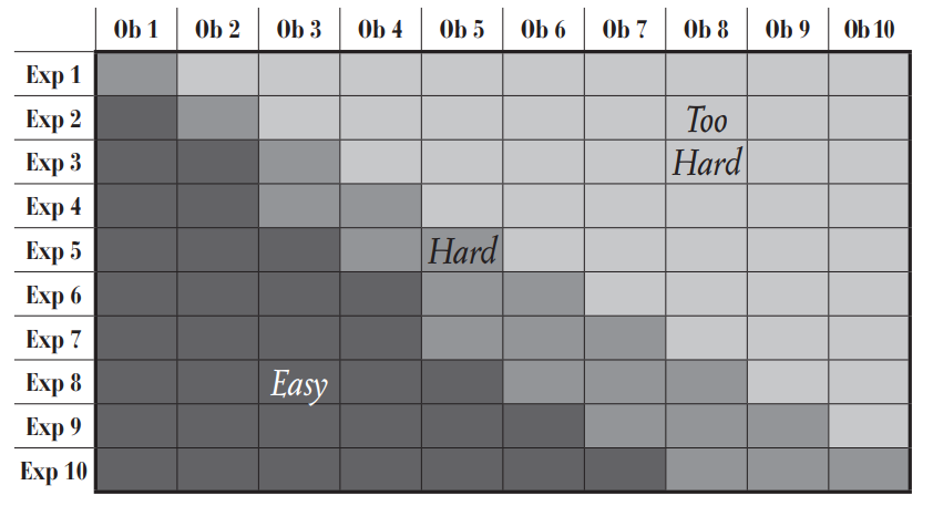
On page 15 of the Burning Wheel Gold Revised we see the table of difficulties shown in Fig. 1. (While "the" is technicaly part of the title, since references to Burning Wheel on its own website do not include "the", I will henceforth dispense with its usage, especially as it's often awkward sounding.) You can get this section of the book for free and see for yourself here. This is a handy-looking table for judging which rolls are of various levels of difficulty. But is it consistent? That is, do all "Easy'' rolls succeed with higher probability than all "Hard'' rolls and likewise, do all "Hard" rolls succeed with higher probability than "Too Hard'' rolls?

Fig. 1: Burning Wheel difficulties

To find out, we'll calculate all the relevant probabilities. In Burning Wheel, you roll a number of six-sided dice equal to the exponent of the skill, which may be increased by various factors. Note that this difficulty table refers to the exponent, not the total number of dice rolled, though. A roll using five dice is often abbreviated 5D. For a black shade skill each die that results in a 4, 5, or 6 is counted as a success. (There are three shades: black, gray, and white, which affect which values on each die count as a success.) If you roll a number of successes equal to the obstacle (abbreviated Ob), then you succeed at the roll. For each die that you roll, you get one success with probability 0.5 and no successes with probability 0.5.

Let's first calculate the probability mass function (pmf) of the number of successes rolled as a function of the number of dice rolled. I've already stated what it is for 1D. Now, let's expand that. Consider the case with two dice. Each die can get a success, so we'll get between 0 and 2 successes. Let's assign the probability of success on a single die as $p=0.5$. To get 0 successes, both dice must fail, which occurs with probability $(1-p)^2 = 0.5^2=0.25$. To get 2 successes, both dice must succeed, which occurs with probability $p^2 = 0.5^2=0.25$ also. All that remains is getting 1 success, which thus must occur with probability $1-0.25-0.25=0.5$. The other way to look at it is that we need one success and one failure, but they can come the two dice in any valid combination. This is occurs with probability $p \cdot (1-p) \cdot n_1$, where $n_1$ is the number of ways to select 1 success die and 1 traitor die (Burning Wheel terminology for a failed die). Since we are assigning all dice as either success or traitor, this is equivalent to picking just the successes (the traitors defined by all those which are not successes). We know that the number of ways to select 1 success die out of 2 dice is 2 choose 1, or $\binom{2}{1} = 2$. Thus, the probability of one success on two dice is,
\begin{align}
\binom{2}{1} \cdot p \cdot (1-p) &= 2 \cdot 0.5 \cdot 0.5 \\
&= 0.5,
\end{align}
matching our previous calculation method. We can use this as a prototype for a general formula. In general for a roll of $n$ dice, where the random variable $S$ represents the number of successes, to get $s$ successes we'll have the general formula for the pmf, $f_S(s) = P(S=s)$, as follows.
\begin{align}
f_S(s) &= \binom{n}{s} \cdot p^s \cdot (1-p)^{n-s}
\end{align}
Here we select $s$ dice to succeed out of $n$ total, which we can do in $\binom{n}{s}$ different ways. Then those $s$ dice must all succeed, which occurs with probability $p^s$, and the remaining $n-s$ dice must all fail, which occurs with probability $(1-p)^{n-s}$. This is known as a binomial distribution. For $n$ dice, we can get from 0 to $n$ successes, which is the range over which this equation is valid. For values above and below this, it's not possible to get that number of successes, and thus the probability is zero. This indicates that at least part of Burning Wheel's table is consistent: "Too Hard" refers to the cases where the probability is 0.

The next step is to compute the probability of getting enough successes on the dice rolled to pass the test. Unfortunately, I don't know a meaningful way to come up with a meaningful closed form solution for this. So, instead, we'll just have to sum the pmf over the range of values that pass. If the Ob is such that we need $o$ successes to pass a test with $n$ dice, then we n
eed to add up the pmf from $o$ to $n$. We need at least $o$ successes and can get at most $n$.
\begin{align}
P(\text{pass}) = \sum_{s=o}^{n} f_S(s)
\end{align}
I've computed these and plotted them in Fig. 2 on top of a color coding matching the difficulty categories printed in Burning Wheel. Note the orientation is different, higher exponents are on top. This is both because I'm thinking of this as a plot instead of a table and because my plotting tool puts it in this order by default. As you can see the difficulties are not consistent. Probabilities of 0.5 are categorized as both easy and hard (Exp 1 vs.\ Ob 1, 3 Exp vs.\ Ob 2) as well as probabilities of 0.25 (Exp 2 vs.\ Ob 2, Exp 9 vs. Ob 6). Probability 0.25 is listed as "Easy" while probability 0.5 is "Hard''.

Fig. 2: Burning Wheel probabilities of passing tests colored by difficulty

In Fig. 3 is a modified figure colored by the probabilities, in which it's easier to see that the slope of constant probabilities is higher than that indicated by the Burning Wheel difficulty table. For example, if we track probably 0.5, we can see that for every increase of 1 in the obstacle, the number of dice needs to increase by 2 to maintain the same probability of passing the test. Is this a real phenomenon, or is it happenstance or just some artifact of rounding in the values shown? This is indeed the actual pattern. The pmf is symmetric, since $S$ is a sum of symmetric random variables (the individual die rolls), as the probability of getting a success or failure on each die is equal. The pmf of successes is the same as the pmf of traitors. There are two cases of symmetry for a discrete random variable: either there is a single center value or a pair of center values. In the case of a pair of center values, that means that the number of possible successes can be put into two groups of equal probability. Thus, when the pmf is summed from the higher center value to the maximum, the result is 0.5. Since the range of possible successes ranges from 0 to $n$, there are $n+1$ possible values. For odd $n$ this is an even number of possibilities, which can be evenly split into two groups. This is why we see that for all odd $n$, the probability of getting $\frac{n+1}{2}$ successes is 0.5.

Fig. 3: Burning Wheel probabilities of passing tests colored by probability

Given that the difficulties listed are not consistent, I see two possibilities. The first possibility, that the author, Luke Crane, doesn't know what the probabilities are. However, we know that this is not the case. In the Monster Burner, there is a table of probabilities (a supplement to an earlier edition of the game, the Codex may have something similar). These are listed as approximate fractions, so I've computed the decimal values (interpreting better than $\frac{9}{10}$ as 1), as shown in Fig. 4. It's hard to compare a large number of values displayed like this. To evaluate the error, I've calculated the difference between the passing probabilities that we calculated and the approximate values in the Monster Burner and plotted them in Fig. 5. The maximum error magnitude is about 0.07 and most are less, so that approximate values are quite good.

Fig. 4: Monster Burner approximate probabilities

Fig. 5: Monster Burner approximation error

The second possible explanation is that these difficulties are meant to have some meaning other than the probability of passing a test. By looking at the advancement table from page 41 we can see the same information presented differently and over a wider range of values. Certain numbers of each type of test are needed to advance skills, which may or may not map to equal probabilities of success depending on the desired properties of the game.

Fig. 6: Burning Wheel advancement

How replayable is Onitama using the 16 move cards in the base game?

Note: there are errors contained in this post as described in the comments below.  See errata here.

First, let me opine on the faulty tacit assumption of the question, namely that replayability is proportional to the possible number of initial states. Two examples show why this is wrong. First, chess, which has a single starting state but a large amount of replayability. Second, look at the card game War (though I learned it where you put three cards face down to spell W A R), where there are many ways that the cards could be distributed between the two players, but there are no choices.

So let us instead answer the question of how many initial states there are in Onitama.

In every game of Onitama, 5 out of the total 16 unique cards are used. I emphasize that the cards are unique, because it matters whether or not we can distinguish between them. Suppose we draw the 5 cards one at a time. For the first card, there are 16 possibilities. When selecting the second card there is one less card, so there are 15 remaining possibilities. This continues until the the fifth card, for which there are $16-4=12$ possibilities. Putting this together, the number of ways in which to draw 5 cards out of 16 unique cards, $n_0$, is given by the following equation.
\begin{align}
n_0 &= 16 \cdot 15 \cdot 14 \cdot 13 \cdot 12 \\
&= 524160
\end{align}
That is a lot of ways. But if we're interesting in the number of sets of 5 cards then we've over counted. For example, we've counted drawing Ox, Elephant, Tiger, Rabbit, then Cobra as distinct from Cobra, Rabbit, Elephant, Tiger, then Ox. To look at the number of combinations we have to divide our previous result by the number of ways we can order the selected 5 cards. Similar to selecting the cards above, we can select the 5 cards one at a time to determine the number of ways to order them. This works out to be the following.
\begin{align}
5! &= 5 \cdot 4 \cdot 3 \cdot 2 \cdot 1 \\
&= \prod_{i=1}^5 i
\end{align}
We say this as "five factorial" and it is equal to the product of all whole numbers from 1 to 5, or in general,
\begin{align}
n! &= \prod_{i=1}^n i .
\end{align}
Thus, the number of ways to select a set of 5 cards out of 16 unique cards is,
\begin{align}
n_1 &= \frac{16 \cdot 15 \cdot 14 \cdot 13 \cdot 12}{5!} \\
&= 4368.
\end{align}
This number of combinations is often said as "16 choose 5'', and can be written as follows, depending on the type of notation used.
\begin{align}
n_1 = \,_{16} C_5 = \binom{16}{5} = \frac{16!}{(16-5)! \cdot 5!}
\end{align}
While this is the number of ways to select a set of 5 cards out of 16, it is not the number of initial states in Onitama. This is because the location of the 5 cards matters, but in a particular way such that $n_0$ is not the number we're looking for. Each player starts with a hand of two cards, but whether those two cards are Ox and Cobra or Cobra and Ox doesn't matter. That means we have three distinct locations that these five cards go, two of which each hold two cards.

What about the two players? Are they interchangeable as well? In some sense yes, in some sense no (people are, of course, not interchangeable). We aren't going to count the number of starting states based on who is playing the game, as it doesn't seem to make sense that the number of states would depend on the world population. On the other hand, it does matter as to whether blue or red has a given pair of cards, since either blue or red makes the first move, as determined by the fifth card. Thus, swapping the cards in the blue and red players' hands gives a different starting state, as the first player has different options.

Given these constraints, we can find the number of ways to assign the 5 selected cards to the two hands and the extra move card. We can do this by taking the existing $5!$ orderings, but then divide by 2 in consideration of the fact that the order of drawing the blue player's hand doesn't matter, and then divide by 2 again because the order of drawing the red player's hand doesn't matter. This works out to,
\begin{align}
\frac{5!}{2 \cdot 2} &= 5\cdot 3 \cdot 2 = 30,
\end{align}
ways to meaningfully arrange the 5 selected cards. For each set of 5 cards, we have 30 ways to arrange them. Thus, to get the total number of initial configurations we multiple the number of ways to select 5 cards by the number of ways to arrange 5 cards into the two hands and extra card.
\begin{align}
n_2 &= \binom{16}{5} \cdot \frac{5!}{2 \cdot 2} \\
&= \frac{16!}{(16-5)! \cdot \require{cancel}\cancel{5!}} \cdot \frac{\require{cancel}\cancel{5!}}{2 \cdot 2} \\
&= \frac{16 \cdot 15 \cdot 14 \cdot 13 \cdot 12}{2 \cdot 2} \\
&= 131040
\end{align}

However, there's one more wrinkle left. To see it, we have to look at the cards themselves. You can see a picture of them here. Half of the cards are symmetric (Tiger, Crab, etc.) while the other half are asymmetric and come in pairs. Frog is the mirror of Rabbit. A game with four symmetric cards and an asymmetric card is essentially the same as a game with those same four symmetric cards and the mirror of the asymmetric card. They're isomorphs of each other. Actually, there's a little wrinkle to that fact, which is that the mirrored cards all have opposite starting colors. This doesn't affect the number of unique starting positions, just which ones are isomorphs of each other. For example, if blue has Tiger and Crab, red has Monkey and Crane, and the extra card is Frog (red starts), then the isomorphic game is blue has Monkey and Crane, red has Tiger and Crab, and the extra card is Rabbit (blue starts). We've just swapped red and blue, left and right, otherwise it's the same.

Next, we need to determine how many initial positions have isomorphs. Expanding from the specific example, above, we're looking for cases where there's at least one asymmetric card, but not its mirror image. Let's count the number of sets of 5 cards that fulfill this condition. We'll first select one of the 8 asymmetric cards randomly. The rest of the cards can be anything except the mirror to the first selected card. That means we are choosing 4 cards out of 14 options, as there are fifteen cards left but one is off limits. The number of ways to do this is,
\begin{align}
n_3 &= 8 \cdot \binom{14}{4} \\
&= 8 \cdot \frac{14!}{(14-4)! \cdot 4!}\\
&= 8008 .\\
\end{align}
We only want to keep half of these, so the number of ways to select 5 cards, excluding isomoprhs is as follows.
\begin{align}
n_4 &= n_1 - \frac{n_3}{2} \\
&= \binom{16}{5} - \frac{8}{2} \cdot \binom{14}{4} \\
&= \frac{16!}{(16-5)! \cdot 5!} - 4 \cdot \frac{14!}{(14-4)! \cdot 4!}\\
&= \frac{16!}{11! \cdot 5!} - 4 \cdot \frac{14!}{10! \cdot 4!}\\
&= \frac{16!}{11! \cdot 5!} - 4 \cdot \frac{11 \cdot 5 \cdot 14!}{11! \cdot 5!}\\
&= (16 \cdot 15 - 4 \cdot 11 \cdot 5 ) \cdot \left ( \frac{14!}{11! \cdot 5!} \right )\\
&= (240 - 220) \cdot \left (18.2 \right )\\
&= 364
\end{align}
To get the number of initial positions with isomorphs, we need to multiply by $\frac{5!}{2 \cdot 2}$ as before.
\begin{align}
n_5 &= n_4 \cdot \frac{5!}{2 \cdot 2} \\
&= \left (\binom{16}{5} - \frac{8}{2} \cdot \binom{14}{4} \right ) \cdot \frac{5!}{2 \cdot 2} \\
&= 364 \cdot 30 \\
&= 10920
\end{align}

How can I use a d20 in Dungeon World?

The basic die mechanic in Dungeon World involves rolling 2d6. A total result of 6 or less results in a failure, 7 through 9 in a partial success, and 10 or more in a success. (What each of these events entails is detailed by the Move that called for a roll.) What's the probability of each event?  We could compute them directly (or even count them), but because there are a couple of cases here (and because we're going to be doing more calculations shortly) it will be helpful to base our calculations on the cumulative distribution function (CDF) of the total result of rolling 2d6. This will make our initial calculation somewhat belabored, but will serve as a framework for subsequent calculations.

The CDF is a function associated with a random variable that tells us the probability of getting a certain number or less. It's usually notated as $F(x)$, or $F_X(x)$, where $X$ is the associated random variable, so we write it's definition as,
\begin{align}\label{eq:def:cdf}
F_X(x) = P(X \leq x).
\end{align}
We'll play a little loose with notation, in order to write our equations with a little more meaning, and write the CDF of the sum of rolling 2d6 as $F_\mathrm{2d6}(x)$. The probability of a failure is $P(\mathrm{2d6} \leq 6)$, which by definition of the CDF is $F_\mathrm{2d6}(6)$. The probability of a partial success is $P(6 <\mathrm{2d6} \leq 9)$. How can we write this in terms of the CDF?  Recall that the probability of disjoint, or mutually exclusive, events add. That means we can break up $P(\mathrm{2d6} \leq 9)$ as follows
\begin{align}
P(\mathrm{2d6} \leq 9) = P(\mathrm{2d6} \leq 6) + P(6<\mathrm{2d6} \leq 9).
\end{align}
Which we can rearrange as
\begin{align}
P(6<\mathrm{2d6} \leq 9) =  P(\mathrm{2d6} \leq 9) - P(\mathrm{2d6} \leq 6).
\end{align}
Substituting in our definition for the CDF, we have
\begin{align}
P(6<\mathrm{2d6} \leq 9) =  F_\mathrm{2d6}(9) - F_\mathrm{2d6}(6).
\end{align}
Similarly, we can find an equation for the probability of success in terms of the CDF.
\begin{align}
P(9<\mathrm{2d6} \leq 12) =  F_\mathrm{2d6}(12) - F_\mathrm{2d6}(9).
\end{align}
However, the maximum possible result of rolling 2d6 is 12. The probability of getting the maximum value or less is 1, so the value of the CDF at 12 is 1.
\begin{align}
F_\mathrm{2d6}(12) = P(\mathrm{2d6} \leq 12) = 1.
\end{align}
Thus, we can simplify the probability of a success as,
\begin{align}
P(9<\mathrm{2d6} \leq 12) =  1 - F_\mathrm{2d6}(9).
\end{align}
To summarize, the probabilities of our three events of interest are
\begin{align}
P(\mathrm{fail}) &= F_{\mathrm{2d6}}(6) \\
P(\mathrm{partial \ success}) &= F_{\mathrm{2d6}}(9) - F_{\mathrm{2d6}}(6) \\
P(\mathrm{success}) &= 1 - F_{\mathrm{2d6}}(9).
\end{align}

What does the CDF look like for our 2d6 roll?  It looks like Fig. 1.  We derived the result previously here.  Let's compare it to 1d20.

Fig. 1: Cumulative distribution function (CDF) of 2d6 and 1d20.

We can read off the values from the plot, or use the equations we derived.
\begin{align}
P(\mathrm{fail}) &= F_{\mathrm{2d6}}(6) \approx 0.417\\
P(\mathrm{partial \ success}) &= F_{\mathrm{2d6}}(9) - F_{\mathrm{2d6}}(6) \approx 0.833 - 0.417 = 0.416 \\
P(\mathrm{success}) &= 1 - F_{\mathrm{2d6}}(9) \approx 1 - 0.833 = 0.167
\end{align}
Note that our approximate values for failure and a partial success came out differently due to how we did the rounding, but they're really the same probability. You can trust me, or do the math yourself to confirm. I advise the latter.

There are two things that stand out about the differences in the CDF of 2d6 compared to 1d20. First, the ranges are different. We can fix this by applying a linear transform, which we'll do shortly. The second is that the shapes of the CDFs are different. Unfortunately, there's no getting around this. We'll just try to line them up as nicely as possible and see how it turns out.

There are a few different ways we could approach generating a mapping from the 1d20 result in order to emulate 2d6. Perhaps the simplest is to just line up the "end points''. They're not really end points, though, since the CDF is really defined over all real numbers. (Even though I haven't plotted it as such. I've neglected both to show the stair-casing and to show values beyond results that are actually possible to roll.)  Let's do this. Here we want to map 0 to 1 and 20 to 12. We can treat those as to $x$-$y$ pairs that define a line. So if we have mapping in the form $y = mx + b$, then
\begin{align}
12 &= m \cdot 20 + b \\
1 &= m \cdot 0 + b.
\end{align}
This works out to be easy to solve, and we don't even have to bother learning some basic linear algebra. From the second equation we see that $b=1$. Plugging that result into the first equation we find,
\begin{align}
12 &= m \cdot 20 + 1 \\
11 &= m \cdot 20 \\
m &= \frac{11}{12}.
\end{align}
So we can emulate 2d6 with a 1d20 by taking the result of the d20 and putting it through the following equation.
\begin{align}
X_\text{fake 2d6} = \frac{11}{20} \cdot X_\text{1d20} + 1
\end{align}
A comparison of a real 2d6 and our fake 2d6 CDF is shown in Fig. 2.

Fig. 2: Comparison of CDF of fake 2d6 and real 2d6.

Now that we've mapped the 1d20 roll onto the 2d6 roll, we can map the limits for failure, partial success, and success back onto the 1d20 directly, so that we don't have to do this awkward linear transform for each roll. We have to do a little invention, because when we map from 1d20 to 2d6 we got numbers in between the previous limits. For example, rolling a 10 on 1d20 maps to $\frac{11}{20}\cdot 10 + 1= 6.5$, which is exactly between the limits for failure and partial success. It's a design decision as to which direction to put the limit for 1d20. Let's put it into partial success. Similarly, rolling a 15 and 16 on 1d20 map to 9.25 and 9.8, respectively, on 2d6. While these are between the limits (9 and 10) for partial success success, they are more clearly on either side of the midpoint (9.5). Thus, we can define the limits as follows.
\begin{alignat}{2}
1 \leq &X_\text{1d20} \leq 9 &&\rightarrow \text{fail} \\
10 \leq &X_\text{1d20} \leq 15 &&\rightarrow \text{partial success} \\
16 \leq &X_\text{1d20} \leq 20 &&\rightarrow \text{success}.
\end{alignat}
We can compute the probabilities associated with this mapping as follows.
\begin{align}
P(\mathrm{fail}) &= F_{\mathrm{1d20}}(9) \\
&= 0.45 \\
P(\mathrm{partial \ success}) &= F_{\mathrm{1d20}}(15) - F_{\mathrm{1d20}}(9) \\
&= 0.3 \\
P(\mathrm{success}) &= 1 - F_{\mathrm{1d20}}(15) \\
&= 0.25 \\
\end{align}
These do sum to one, indicating we've done the math correctly. However, the probabilities are quite different than what we had when we started with 2d6. Failure is fairly close, but partial success is much less likely, and success is much more likely. This is likely to notably affect the game. So let's look at another approach.

One possible improvement would be to alter our mapping function. One way would be to calculate the so-called best-fit line. (I use "so-called'' because depending on what the criteria for best is in a particular case, there may be a better line than the best-fit line.) This is the line for which the mean-squared error is minimized.

Another approach would be to look at the points we really care about—at 6 and 9—and just do a fit based on those. Or, put it another way, let's look at the probabilities of the three results with 2d6, and find what thresholds best match those probabilities. For our 1d20, all outcomes have a probability which is a multiple of $1/20=0.05$, so if we just round our probabilities to the nearest multiple of 0.05, and then look at what thresholds give us those probabilities, we can find the transform. Actually, we'd be done, since what we really want is the thresholds. However, the transform will be useful for later.
\begin{align}
P(\mathrm{fail}) &\approx 0.417 \rightarrow 0.4\\
P(\mathrm{partial \ success}) &\approx 0.416 \rightarrow 0.4\\
P(\mathrm{success}) &\approx 0.167 \rightarrow 0.15
\end{align}
Unfortunately, when we round to the nearest 0.05, the resulting probabilities don't add up to 1. That is, $0.4+0.4+0.15=0.95$. Again, it's a design decision as to where to put this leftover 0.05 probability. Personally, I'd put it into partial success, since that's usually the most interesting result. (Indeed others who had done d20 hacks of Dungeon World agree with me—or, perhaps, I agree with them—and use this breakdown. Unfortunately, I can't find a working link right now.)
\begin{align}
P(\mathrm{fail}) &= 0.4\\
P(\mathrm{partial \ success}) &= 0.45\\
P(\mathrm{success}) &=0.15
\end{align}
To achieve these probabilities, we need to have a number of possible results on 1d20 correspond to each outcome equal to the probability of that outcome divided by 0.05. We'll keep them in order so that
\begin{alignat}{2}
1 \leq &X_\text{1d20} \leq 8 &&\rightarrow \text{fail} \\
9 \leq &X_\text{1d20} \leq 17 &&\rightarrow \text{partial success} \\
18 \leq &X_\text{1d20} \leq 20 &&\rightarrow \text{success}.
\end{alignat}
What complicates our situation is that sometimes there are modifiers to the roll. These modifiers can range from $-3$ to $+4$. The $+4$ comes from a stat giving a $+3$ and also having $+1$ from another effect. In Fig. 3 we see plots of the probabilities of the three outcomes in Dungeon World (using 2d6) with these modifiers. Thus, while we've got the thresholds for unmodified rolls, we still need to know how to map the modifiers to a 2d6 roll to modify the 1d20 roll.

Fig. 3: Probabilities of a roll in Dungeon World.

To address this, we'll do a mapping using these probabilities. Because of rounding, we have a little bit of wiggle room. Let's look at two lines that bound our possibilities. We could either map 8 to 6 or 9 to 7, and either 17 to 9 or 18 to 10. Each combination gives us two equations with two unknowns to solve for. Let's plot these four points. Let's consider the combination that gives us the largest slope.
\begin{align}
6 &= m \cdot 8 + b\\
10 &= m \cdot 18 + b
\end{align}
We can write this in matrix notation,
\begin{align}
\begin{bmatrix}
6 \\
10 \\
\end{bmatrix}
& =
\begin{bmatrix}
8 & 1 \\
18 & 1 \\
\end{bmatrix}
\cdot
\begin{bmatrix}
m \\
b \\
\end{bmatrix}
\end{align}
Now let's assign the matrices variables, so we can rearrange to solve for what we want.
\begin{align}
\mathbf{A} &=\mathbf{B} \cdot
\begin{bmatrix}
m \\
b \\
\end{bmatrix} \\
\mathbf{B}^{-1} \cdot \mathbf{A} &= \mathbf{B}^{-1} \cdot \mathbf{B} \cdot
\begin{bmatrix}
m \\
b \\
\end{bmatrix} \\
\begin{bmatrix}
m \\
b \\
\end{bmatrix}
&= \mathbf{B}^{-1} \cdot \mathbf{A} =
\begin{bmatrix}
0.4 \\
2.8 \\
\end{bmatrix}
\end{align}
Note that we have to be a bit careful with how we do operations with matrices. Matrix multiplication isn't commutative. That is, the order matters, which is why $\mathbf{B}^{-1}$ is the left-most term above. I've glossed over the details here, for which I'm somewhat sorry, because the matrices aren't our focus here. The above should compute easily enough in tools to handle such things (e.g. python). Or, you could solve the two equations manually.

Now let's consider a combination that gives us the smallest slope.
\begin{align}
7 &= m_2 \cdot 9 + b_2\\
9 &= m_2 \cdot 17 + b_2
\end{align}
Here, I'll elide even more of the steps and get to the result.
\begin{align}
\begin{bmatrix}
7 \\
9 \\
\end{bmatrix}
& =
\begin{bmatrix}
9 & 1 \\
17 & 1 \\
\end{bmatrix}
\cdot
\begin{bmatrix}
m_2 \\
b_b \\
\end{bmatrix} \\
\mathbf{A_2} &=\mathbf{B_2} \cdot
\begin{bmatrix}
m_2 \\
b_2 \\
\end{bmatrix} \\
\mathbf{B_2}^{-1} \cdot \mathbf{A_2} &=
\begin{bmatrix}
m_2 \\
b_2 \\
\end{bmatrix} \\
\begin{bmatrix}
m_2 \\
b_2 \\
\end{bmatrix}
&=
\begin{bmatrix}
0.25 \\
4.75 \\
\end{bmatrix}
\end{align}
These two lines are plotted on top of the mapped thresholds in Fig. 4. The corresponding probabilities are plotted in Fig. 5.

Fig. 4: Mapping thresholds.

Fig. 5: Mapping thresholds onto 2d6 CDF.

What really matters here is the slopes, which range from $1/m=1/0.4=2.5$ to $1/m_2=1/0.24=4$. This means that we can use the thresholds we computed, and then map each $+1$ modifier on 2d6 to somewhere between $+2.5$ to $+4$ on 1d20. Practically, we should limit this to integer values. Thus we can consider $+2$, $+3$, and $+4$ to 1d20 per $+1$ to 2d6. These three cases are plotted in the three figures below.

Fig. 6: Probabilities of a roll where $+1$ on 2d6 becomes $+2$ on 1d20.

Fig. 7: Probabilities of a roll where $+1$ on 2d6 becomes $+3$ on 1d20.

Fig. 8: Probabilities of a roll where $+1$ on 2d6 becomes $+4$ on 1d20.

Looking at these plots we can see that there's some level of trade off between them. It looks to be overall the best when we map $+1$ to $+3$, however there is one property that stands out. With even the minimum $-1$ penalty using a 2d6 becomes $-3$, which means that the probability of success becomes 0. To rectify this, we can invoke a rule from Dungeons and Dragons: rolling a natural 20 and 1 result in automatic success and failure, respectively. With this rule incorporated we see the probabilities plotted in the figure below, which does a nice job of matching the shapes, but also preserves a non-zero chance of both success and failure with small modifiers, as in Dungeon World using 2d6.

Fig. 9: Probabilities of a roll where $+1$ on 2d6 becomes $+3$ on 1d20 and special treatment of 1 and 20.