Should everyone always lose semi-coop games?

Unfortunately, in order to answer this question, we have to do a bit of taxonomy first, as "semi-coop", short for semi-cooperative, means different things to different people.

Some people call hidden team games like Battlestar Galactica and/or cooperative games with a possible traitor like Shadows over Camelot semi-coops. I can see the motivation for this as they look like a "cooperative, but ..." game, yet it doesn't seem necessary to differentiate these from other team games like Space Cadets: Dice Duel, Codenames, and The Resistance.

Instead, we are talking about games like CO₂, Legendary, and Dead of Winter. The through-line seems to be that these are games where players do not always win together (like a cooperative game), but they may all lose together. However, that definition includes games like Galaxy Trucker, which I don't think anyone would consider a semi-coop. A more precise definition would be that there is a condition that if not met means that none of the non-traitor players are eligible to win and instead lose. I specify non-traitor because many, but not all, of these games feature a traitor, who is essentially on a team with the game trying to make the rest of the players lose.

Within this definition I see three types of semi-coop, which have important distinctions that we'll get to.

In type I semi-coops, or single-winner semi-coops, either all players lose or one player wins while all other players lose. Examples include CO₂ (in "mostly competitive" mode), Robin Hood and the Merry Men, Castaways, and Divided Republic. Examples that include a possible traitor are AuZtralia, Homeland, and Republic of Rome (which has an opt-in traitor).

In type II semi-coops, or group-win semi-coops, there are two types of winning. Either all players lose or all players win, but if all players win there is also an individual winner. Examples include Legendary, Castle Panic (although it only uses the word "win" for the group win), Arkham Horror (group win plus "honorary title of First Citizen of Arkham"), Horizon Zero Dawn (although the terminology is confusing "Although all players have won..., the player with the most victory points...emerges as the winner of the game"), and Tomorrow (mentions "win" for both, but in separate sections of the rulebook). Archipelago is an example with a possible traitor.

Type III semi-coops, or separate-goal semi-coops, have separate win conditions for each player in addition to the group loss. An example is Forgotten Waters. Examples with a possible traitor include Dead of Winter, Nemesis, and New Angeles. Dead of Winter labels itself as a "meta-cooperative" game, but the term doesn't seem to have caught on, though it may be useful to describe type III semi-coops.

Games that don't fit this definition but some may call semi-coops include Cutthroat Caverns, Crisis, Bag of Dungeon (using an optional advanced rule), Hellapagos (whoever gets rescued wins, which can be any subset of players), Fog of Love (each player's performance is determined individually), Pax Emancipation (which has a first phase after which the game may end with any number of players may win except all, as well as a possible second phase which is purely competitive) and Core Space (which has the odd combination of a group win if an objective is completed and an individual win if it is not). While these games do feature the possibility of everyone losing, this is usually still determined on a per-player basis.

Type I: single-winner semi-coops

Let's look at a simplified model of a three player type I semi-coop game. Each player has two moves and chooses simultaneously: cooperate (C) or defect (D). If at least two players cooperate, this prevents the all lose scenario. If one player defects, that player is the winner. If all players cooperate, then the winner is randomly select from them.  This is depicted in Table 1, where each row represents an outcome based on the first player's move (P1), while each column represents the combined moves of the second and third players (P2 & P3).

\begin{align*} \begin{array}{c |c|c|c} \text{P1 \\P2 & P3} & 2 D & 1D, 1C & 2C \\ \hline D & \text{All lose} & \text{All lose} & \text{P1 wins} \\ C & \text{All lose} & \text{P2 or P3 wins} & \text{P1 may win} \end{array} \end{align*} 

Table 1: A simple type I semi-coop game

Type I semi-coops have the issue that the best move is to defect, as defecting is a weakly dominant strategy, meaning that defecting is sometimes better but never worse than cooperating. This is perhaps more clear in Table 2, which is focused on the first player. Additionally, if players put any positive value to have fellow players also lose (that is, any preference for all lose to someone else wins), then defecting is even more incentivized, but remains a weakly dominant strategy.

\begin{align*} \begin{array}{c |c|c|c} \text{P1 \P2 & P3} & 2 D & 1D, 1C & 2C \\ \hline D & \text{Lose} & \text{Lose} & \text{Win} \\ C & \text{Lose} & \text{Lose} & \text{May win} \end{array} \end{align*}

Table 2: First player's outcomes simple type I semi-coop game

Note that this model only holds if two players cannot easily spoil the victory of another. Additionally, it assumes individual victory and avoiding group loss are at odds with each other. This trade-off is not inherent. For example, suppose you have a game where players earn points throughout the game and all players lose if the sum of the points of all players is not sufficiently high. Now, consider two metrics for individual victory. In the first, the player with the fewest number of points is the individual winner. Here, as long as you lack the ability to manipulate other player's points, the lessons we learned above hold and we wouldn't expect there to be a winner (depending on the total point threashold), as all players tries to minimize their own scores. However, in the second metric, the player with the most number of points is the individual winner. Here, actions that avoid a group loss and obtain individual victory are likely perfectly aligned (there are likely some exceptions due to interactions with other players). Since players are trying to maximize their own scores to be the individual winner, the group loss condition is easily avoided. Of course, in such a situation, you may ask why a group loss condition is included in the game. (While I doubt such a game exists, you could include the rule to avoid dominant strategies that end the game very quickly and are not satisfying in some way. There may be better solutions than making the game semi-cooperative.) The defect or cooperate paradigm does not match with this second metric for an individual win.

Type II: group-win semi-coops

Let's move onto the more interesting type II semi-coop. Table 3 shows another model of a simple simultaneous-play semi-coop game. This time we've adjusted the values both to represent a type II semi-coop, but also to look at the payoffs for the first player, so that we can make use of a game theory analysis. We will assume that all lose is valued at 0, while group win or all win ($AW$) and individual win ($IW$) each have some positive unknown value (but common to all players).

\begin{align*}
\begin{array}{c |c|c|c}
\text{P1 \P2 & P3} & 2 D & 1D, 1C & 2C \\ \hline
D & 0 & 0 & AW+IW \\
C & 0 & AW &AW+\frac{1}{3}IW
\end{array}
\end{align*}

Table 3: A simple type II semi-coop game

First, let's acknowledge some fragility to this system. Akin to how competitive games can break down if any of the players are not trying to win (it seems relevant to quote Reiner Knizia: "Remember: When playing a game, the goal is to win, but it is the goal that is important, not the winning..."), semi-cooperative games can break down if players do not accept the payoffs given by the game. While competitive games have their payoffs generally accepted and understood by most people, semi-cooperative games are more rare, especially type II semi-coops, which have multiple types of winning. Some players may ignore one or the other type of winning. If $IW$ is valued at 0, then the game is essentially cooperative, and all players will cooperate as it is a weakly dominant strategy. If $AW$ is valued at 0, then the game reverts to a type I. Some people also reject the idea that a group win is better than a group loss in a type II semi-coop (the interpretation is that in the case of a group loss, all players do as well as each other and so the game ends in a draw, which is preferable to a group win where you are losing to another player; the latter is interpreted as a simple loss), essentially valuing $AW<0$. In that case, as in type I, defecting is a weakly dominant strategy (it's better if exactly one other player cooperates, but doesn't matter if both others either cooperate or defect together). Under such a valuing of the outcomes the game breaks down as it does in a Type I semi-coop. Conversely, players of a Type I semi-coop may value avoiding the all-lose condition such that they effectively add a group win, turning it into a type II semi-coop. We will proceed assuming all players accept the value of both types of winning, while also acknowledging there is some ambiguity in that these games do not specify how much to care about the two types of winning relative to each other.

In this type II semi-coop there is no obviously best move. If both other players defect, it doesn't matter what the first player does. If one other player defects but one cooperates, then cooperation is preferred as this ensures that all win (including player one). On the other hand, if both other players cooperate, then defection is preferred, as that move guarantees obtaining the individual win.

This type II semi-coop has several Nash Equilibria. The first three pure-strategy Nash Equilibria are the cases where one player defects while the other two cooperate. There are three, because there's one for each player being the defector. This is a Nash Equilibrium because no player can do better by changing strategy. Suppose the first player is defecting while the other two are cooperating. This puts us in the third column. The first player is better off with a definite individual win than a one-third chance of an individual win. In both cases, the group win condition is guaranteed. The second and third players each face the choice between a group win and a group loss. Neither can unilaterally do anything to do better given the strategies of the other players. A lesson that we can take from this model is that if you can be the first to convince other players that you either have or will defect, you will likely be the individual winner. As such, these games may have a strong first-player advantage, depending on how quickly a player can establish defection.

Another pure strategy Nash Equilibrium is if all players defect. With all players defecting, the all lose outcome occurs, but no single player is in a position to change it. Here it is evident that the Nash Equilibrium is really about stability not about a how good a set of strategies is. Note that in this situation, though, any player may deviate from a defection strategy without detriment.

There is also a mixed-strategy (a mixed-strategy employs one of a number of pure strategies with a given set of corresponding probabilities) Nash Equilibrium of cooperate and defect. The mix depends on the relative valuing of the different outcomes. To find this Nash Equilibrium, we'll make use of the fact that we know that each component strategy must be a best response and have the same average payout. So the payout of defect and cooperate must be the same. Assume in the equilibrium that each player cooperates with probability $p$, and thus defects with probability $1-p$. The probability that both players 2 and 3 cooperate is $p^2$. The probability that they do one of each is $2 \cdot p \cdot (1 - p)$. Recall that the 2 comes from the fact that either player could be the one that cooperates, so there are two ways that it happens. The payoff for player one are thus as follows.

\begin{align}
u(D) &= p^2 \cdot \left ( AW + IW \right ) \\
u(C) &= 2 p(1-p) \cdot AW + p^2 \cdot \left ( AW +\frac{1}{3} IW \right )
\end{align}

So let's set these equal to find $p$.
\begin{align}
u(D) &= u(C) \\
p^2 \cdot \left ( AW + IW \right ) &= 2 p(1-p) \cdot AW + p^2 \cdot \left ( AW +\frac{1}{3} IW \right ) \\
p^2 \cdot \left (\frac{2}{3} IW \right ) &= 2 p(1-p) \cdot AW \\
p\cdot \frac{2}{3} IW &= 2 (1-p) \cdot AW \\
p\cdot \left (\frac{2}{3} IW + 2AW \right ) &= 2\cdot AW \\
p &= \frac{2 AW}{\frac{2}{3} IW + 2AW}
\end{align}

We can see our earlier conclusions about the simplified cases fall out from this. If $AW=0$, then $p=0$, as we're in the type I semi-coop case. If $IW=0$, then the game is cooperative and $p=1$. For positive values of both AW and IW, though, we find $0 < p < 1$. Note that this works even if having everyone win is valued significantly above having the individual win, as an individual win requires a group win. We can rewrite this based on the ratio of the two values, $r = AW / IW$.

\begin{align}
p &= \frac{2 AW}{\frac{2}{3} IW + 2AW} \\
p &= \frac{2 \frac{AW}{IW}}{\frac{2}{3} + 2\frac{AW}{IW}} \\
\require{cancel}p &= \frac{\cancel{2}\cdot 3 \frac{AW}{IW}}{\cancel{2} + \cancel{2}\cdot3\cdot\frac{AW}{IW}} \\
p& = \frac{3r}{1 + 3r}
\end{align}

This is a monotonically increasing function, as shown in Figure 1, so the more we care about the group win compared to the individual win, the more we cooperate (this is expected and perhaps obvious).

Figure 1: Probability of Cooperation in a Type II Semi-cooperative Game with Equal Player Standing

Suppose we value them equally, such that achieving individual victory has twice the total utility as being part of a group win. This means that we'll cooperate with probability $p=3/4$ or 75% of the time.

Operating under this strategy, we can find the probability that the group wins. This occurs when at most one player defects. The probability that all players cooperate is $p^3$. The probability that one player defects is $3\cdot p^2 \cdot (1-p)$. For $p=3/4$, this means the probability of a group win is,

\begin{align}
P(AW) &= p^3 + 3 \cdot p^2 \cdot (1-p) \\
&= 3p^2 - 2p^3 \\
&= 3 \cdot \left (\frac{3}{4} \right ) ^2 - 2 \cdot \left ( \frac{3}{4} \right ) ^3\\
&\approx 0.84.
\end{align}

This is shown in Figure 2 as a function of the ratio $r$.

Figure 2: Probability of Successful Cooperation in a Type II Semi-cooperative Game with Equal Player Standing

Type II with unequal standing

Now, let's consider a case where the players do not have equal standing. This perhaps models the end of the game. Let's assume players 1, 2, and 3 are in that rank, such that if all cooperate, then player 1 will win. However, if any one player defects (with the other two cooperating) the defecting player wins.

\begin{align*}
\begin{array}{c |c|c|c}
\text{P1 \ P2 & P3} & 2 D & 1D, 1C & 2C \\ \hline
D & 0 & 0 & AW+IW \\
C & 0 & AW &AW+IW \\
\end{array}
\end{align*}

Table 4: A simple type II semi-coop game for player 1 while ahead

Here, for player 1, cooperate is weakly dominant, since the individual win is ensured if all player cooperate. Thus, player 1 likely cooperates.

\begin{align*}
\begin{array}{c |c|c|c}
\text{P2/3 \ P1 & P3/2} & 2 D & 1D, 1C & 2C \\ \hline
D & 0 & 0 & AW+IW \\
C & 0 & AW &AW
\end{array}
\end{align*}

Table 5: A simple type II semi-coop game for players 2 or 3 while behind

However, players 2 and 3 are much more like the earlier analysis. We can check the previous Nash Equilibria to see if they still hold. All defect still is, as well as cases where any one player defects while the other two cooperate. However, player 1 defecting and others cooperating is now a weak Nash Equilibrium, as player 1 is no worse off for cooperating.

Due to the asymmetry introduced, when looking for an updated mixed-strategy Nash Equilibrium, let's say that the first player cooperates with probability $p_1$ and the second and third players each cooperate with probability $p_2$. We can now employ similar techniques as before, however, we'll have more equations as we have a new variable. We'll still assume that $AW$ and $IW$ are valued equally between all players. First, let's look at the payoffs for player 1.

\begin{align}
u(D_1) &= p_2^2 \cdot \left ( AW + IW \right ) \\
u(C_1) &= 2 p_2(1-p_2) \cdot AW + p_2^2 \cdot \left ( AW + IW \right ) \\
u(D_1) &= u(C_1)
\end{align}

From this point, we just do some algebra.

\begin{align}
\require{cancel}\cancel{p_2^2 \cdot \left ( AW + IW \right )} &= 2 p_2(1-p_2) \cdot AW + \cancel{p_2^2 \cdot \left ( AW + IW \right )}\\
0 &= 2 p_2(1-p_2) \cdot AW
\end{align}

Here there are two solutions, $p_2=0$ and $p_2=1$. This is somewhat of a contradiction, as we assumed a mixed-strategy for players 2 and 3, yet here we get pure strategies. If we look at the payoffs for player 1, we see the incorrect assumption that we made: that player 1 plays a mixed strategy. Cooperating is always as good as defection for player 1, and sometimes better. If players 2 and 3 are playing mixed strategies, then we should expect that sometimes one will cooperate and one will defect, which means that the only way for player 1 to have a best response 100% of the time is to cooperate.

Knowing this, we can actually simplify the game from, since we know player 1 will cooperate.

\begin{align*}
\begin{array}{c|c|c}
\text{P2/3 \ P3/2} & D & C \\ \hline
D & 0 & AW+IW \\
C & AW &AW
\end{array}
\end{align*}

Table 6: A simple type II semi-coop sub-game for players 2 & 3 if player 1 cooperates

Again using $p_2$ for the probability of cooperation for only players 2 and 3, we can find the payoffs for each move. We'll repeat the same method of setting the payoffs equal to each other.

\begin{align}
u(D) &= u(C)\\
p_2 \cdot \left (AW+IW \right ) &= AW\\
p_2 &= \frac{AW}{AW+IW}\\
p_2 &= \frac{r}{1+r}
\end{align}

We find a probability of cooperation which is lower than before (assuming the same values of ratio of the value of the group win AW to the individual win IW). For equal values ($r=1$), $p_2=0.5$, only 50%! This makes sense, as there's less incentive now to cooperate. A graphical comparison is presented in Figure 3.

Figure 3: Probability of Cooperation in a Type II Semi-cooperative Game with 2 Players Behind a Leader compared to Equal Standing

However, did this decrease the probability of a group win?

\begin{align}
P(AW) &= p_2^2 + 2\cdot p_2 \cdot (1-p_2) \\
&=2p_2 - p_2^2\\
&=0.75
\end{align}

This did somewhat decrease the probability of a group win, but perhaps not by as much as we might have thought. As shown in Figure 4, there are even some cases where the probability of successful cooperation is higher than with equal standing, although this is only when the group win is valued at a small fraction of the individual win.

Figure 4: Probability of Successful Cooperation in a Type II Semi-cooperative Game with 2 Players Behind a Leader compared to Equal Standing

Type III: separate-win semi-coops

Since type III semi-cooperative games, or meta-cooperative games, do not rank players to determine a winner, there is not the same kind of concept of cooperating vs. defecting as in the analyses we performed thus far. There may still be tension between avoiding the all-lose outcome and achieving personal goals, but this tension is not directly influenced by the situation of other players.

Conclusion

To recap, we saw that in a simple type I semi-coop game, where either all lose or there is one winner, we somewhat expect that all players lose.  (Note that while this may be a strategically unsatisfying play experience, it may be interesting art or commentary.) This is the only Nash Equilibrium and defecting is a weakly dominant strategy. If we add a group win, thus converting to a type II semi-coop, we can avoid this, as there are stable states where all players win. However, this is subject to the strategies employed by the players. If a majority of the players demand to get advantage for the individual win by defecting, then all will lose, and all players defecting is also a Nash Equilibrium. Additionally, even in the case where the group win is achieved, this could be because a certain player is defecting while the others cooperate. Such a condition may be unpleasantly static.  

So the answer is no, as players in a group-win semi-coop may be able to rationally achieve cooperation.

Errata: What's the toughest unit in Memoir '44?

I was preparing to revisit what the toughest unit in Memoir '44 is by looking at it using a Markov chain model. Then I discovered that I had an error in my earlier calculation. I'll fix my calculation and derive the expected number of dice needed to eliminate each type of unit. Recall that I derived the following equation for the expected number of dice needed to eliminate a given unit, $N$, as follows. \begin{align} \mathbb{E} N &= \sum_{n=0}^\infty 1 - F_N(n) \end{align} Here $F_N(n)$ is the CDF of $N$, meaning that $F_N(n) = P(N \leq 0)$. See the previous analysis for the derivation of the CDF. The error came in the range of the summation for $\mathbb{E} N$, which starts at zero. However, my code to the computation stored the CDF starting at $n=1$, since it is known to be 0 at $n=0$; it's impossible to eliminate a unit without rolling any dice. This means that I should add one to the previous estimates, as shown below. \begin{align} \widehat{\mathbb{E} N_\text{infantry}} & \approx 8.000000000000002 \\ \widehat{\mathbb{E} N_\text{armor}} & \approx 8.999999999999932 \\ \widehat{\mathbb{E} N_\text{artillery}} & \approx 11.999998659711212 \\ \end{align} 

Figure 1: Estimating expected value with finite sum

This means that our guess as to the true expected values are below and the updated formula would be $\mathbb{E} N = f/p$. \begin{align} \mathbb{E} N_\text{infantry} & = 8 \\ \mathbb{E} N_\text{armor} & = 9 \\ \mathbb{E} N_\text{artillery} & = 12 \end{align} This makes a lot more sense and perhaps I should have caught the previous error. Without the odd $-1$ hanging off the back end of the equation, this means that the expected value of proportional to the number of starting figures. This makes sense, especially in our one die at a time analysis. If it takes an average of $1/p$ dice to remove one figure, then it should take an average of $f/p$ dice to remove $f$ figures. First, we remove one figure, then the second, and then so on $f$ times. Each time takes an average of $1/p$ dice, so $f/p$ dice in total. The expectation is also inversely proportional to $p$. While clearly in the correct direction, it'll take a little more analysis to establish this precise relationship. If we increase the probability of hitting with each die, it'll decrease the number of dice we need to roll before getting a hit. Let's analysis the expected number of dice rolled to get the first hit, $N_\text{hit}$, for a unit with a probability of getting hitting one die $p$. To get a hit on the $n$-th die, after missing previously, the probability is, \begin{align} P(N_\text{hit} = n) = (1-p)^{n-1} \cdot p. \end{align} While we could use this, we can use the same shortcut to find the expected value as before. \begin{align} \mathbb{E} N_\text{hit} = \sum_{n=0}^\infty P(N_\text{hit} > n) \end{align} The probability that we haven't gotten a hit in $n$ dice, $P(N_\text{hit} > n)$ is the probability that we roll a miss all $n$ times. \begin{align} P(N_\text{hit} > n) = (1-p)^n \end{align} Thus, the expected value is, \begin{align} \mathbb{E} N_\text{hit} = \sum_{n=0}^\infty (1-p)^n . \end{align} This is a familiar infinite series, although it might not be immediately recognizable in this form. If we instead substitute $a = 1-p$ and notice that $a < 1$ for $p > 0$, then it becomes more familiar. \begin{align} \mathbb{E} N_\text{hit} &= \sum_{n=0}^\infty a^n \\ &= a^0 + a^1 + a^2 + a^3 + \ldots \\ & = \frac{1}{1-a} \end{align} This is very similar to the analysis done related to rolling for actions in First Martians. Finally, we substitute back in that $a = 1-p$. \begin{align} \mathbb{E} N_\text{hit} &= \frac{1}{1-a} \\ &= \frac{1}{1 - (1-p)} \\ & = \frac{1}{p} \end{align} Combining this result for a single figure with the previous analysis we find that indeed $\mathbb{E} N = f/p$.

Link: Special Hunt Tiles in War of the Ring

I found the above analysis of the special red and blue hunt tiles in War of the Ring by Ira Fay to be interesting.  Also see the linked simulator here: http://irafay.com/wotr_mordor.php.

For my taste, I'd want to figure out how to do this without relying on a Monte Carlo simulation, but it's probably a lot easier and seems to run pretty fast.

Note: Ira also has several videos on his channel of him going through games of War of the Ring that he goes through and comments on.

Should I roll or use two pawns in First Martians?

In my review of First Martians, I included a table showing the expected number of pawns required for each type of action when rolling (see Table 1). Here's I'll go through the math behind that table. 

Table 1: Expected pawns when rolling for actions

First, let me establish the relevant rules and constraints of the analysis. In general, actions may completed by using two pawns on them for an automatic success, or only using one pawn but having to roll three dice that determine a number of possible outcomes. Some actions require additional dice, which I'll discuss briefly later. The first die determines whether the action succeeds or the player gains two morale tokens (which power special abilities), the second die determines whether or not the character receives a wound, and the third die determines whether the character has an adventure, which entails requesting a the app for the game to explain some additional event which generally harms the character in some way or provides some additional obstacle. Since these are three separate dice being rolled they are all independent and any combination of outcomes is possible. Further, the distributions of the types of sides on the three dice depend on the type of action. Each die determines only one of two sets of outcomes, Table 1 shows the probabilities for the three outcomes of interest: success, wound, and adventure. We'll denote these as $p_s$, $p_w$, and $p_a$, respectively. While morale tokens can be useful, I have ignored them here, as they do not necessarily translate into success in a given action. Next, let's look at how many times we'll have to roll in order to succeed at the action, given by the random variable $N$. A useful way to calculate this for non-negative random variables is the following equation. \begin{align} \mathbb{E} N = \sum_{n=0}^\infty P(N > n) \end{align} While I won't do a full proof, I'll note that there's some discussion of it here. The following illustration will help to see why this is true. We can write $P(N > n)$ in terms of all the relevant $P(N = n)$. \begin{align} P(N>n) &= \sum_{i=n+1}^\infty P(N=i) \\ &=P(N=n) + P(N=n+1) + P(N=n+2) + \ldots \\ \mathbb{E} N &= \sum_{n=0}^\infty \sum_{i=n+1}^\infty P(N=i) \\ \end{align} We can expect and regroup this to see how it's equal to the expected value. \begin{alignat}{9} \mathbb{E} N =& P(N = 1) &&+& P(N = 2) &&+& P(N = 3) &&+& P(N = 4) &&+&\ldots \\ & &&+& P(N=2) &&+& P(N = 3) &&+& P(N = 4) &&+&\ldots \\ & &&& &&& P(N = 3) &&+& P(N = 4) &&+&\ldots \\ &\underbrace{\phantom{P(N = 1)}}_{1\cdot P(N=1)} &&& \underbrace{\phantom{P(N = 2)}}_{2\cdot P(N=2)} &&& \underbrace{\phantom{P(N = 3)}}_{3\cdot P(N=3)} &&+& \underbrace{P(N = 4)}_{4\cdot P(N=4)} &&+& \ldots \\ \end{alignat} This matches the expected value, which is the average, given by the sum of all possible outcomes weighted by the probability that they occur. \begin{align} \mathbb{E} N = \sum_{n=1}^\infty n \cdot P(N = n) \end{align} Here, the number of rolls must be at least one, so the range of the summation is set accordingly. However, note that this also works for random variables which are non-negative ($N\geq 0$) instead of strictly positive ($N>0$), because the 0 term is always zero ($0 \cdot P(N= 0) = 0$). Now let's look at the relevant probabilities in this case. Given a probability of success, $p_s$, we can find the probability that the number of rolls, $N$, is more than $n$. It is the probability that the first $n$ rolls fails, which each occur with probability $1-p_s$. These are independent, so we can multiply all the probabilities together. \begin{align} P(N > n) &= (1-p_s)^n \end{align} Thus, the expected value is, \begin{align} \mathbb{E} N = \sum_{n=0}^\infty (1-p_s)^n . \end{align} This is a familiar infinite series, although it might not be immediately recognizable in this form. If we instead substitute $a = 1-p_s$ and notice that $a < 1$ for $p_s > 0$, then it becomes more familiar. \begin{align} \mathbb{E} N &= \sum_{n=0}^\infty a^n \\ &= a^0 + a^1 + a^2 + a^3 + \ldots \\ & = \frac{1}{1-a} \end{align} If you haven't seen this before, first, let's remember that $a^0 = 1$. \begin{align} \mathbb{E} N &= 1 + a^1 + a^2 + a^3 + \ldots \end{align} Next we can multiple both sides by $a$ and then add 1 to both sides. \begin{align} a \cdot \mathbb{E} N &= a^1 + a^2 + a^3 + \ldots \\ 1 + a \cdot \mathbb{E} N &= 1 + a^1 + a^2 + a^3 + \ldots \\ \end{align} At this point we notice that the right hand side is equal to our original infinite series for $\mathbb{E} N$. From there we can employ some algebra to find the expected value in question. \begin{align} 1 + a \cdot \mathbb{E} N &= \mathbb{E} N \\ 1 &= \mathbb{E} N \cdot (1 - a) \\ \frac{1}{1-a} &= \mathbb{E} N \end{align} Finally, we substitute back in that $a = 1-p_s$. \begin{align} \mathbb{E} N &= \frac{1}{1-a} \\ &= \frac{1}{1 - (1-p_s)} \\ & = \frac{1}{p_s} \end{align} This means that expect to roll 1.2 times and 1.5 times for $p_s = 5/6$ and $p_s = 4/6$, respectively. If this were the only die in consideration, perhaps this would make a good game. In general it would be more efficient to roll, but sometimes it be important to guarantee success now. However, there are two other dice in the picture, related to wounds and adventures. To deal with a wound costs 1 pawn in 1--3 player games and 2 pawns in 4 player games; I'll use the lower 1 pawn cost, even though sometimes a wound can trigger a condition token which usually costs a pawn to remove. Based on my experience with the game (20+ plays), I estimate the cost of dealing with an adventure to average out to about 1 pawn also, though this in more variable. In both cases, you may or may not have to pay these costs. If the game is close to the end, or it affects an abundance resource, you may not have to. However, wounds usually need to be healed to avoid potential death. Any cost here is borne in subsequent rounds, which can make a difference, but is not quantified here. Wounds occur with probability, $p_w$, of $3/6=1/2$ or $2/6 = 1/3$, while adventures occur with probability, $p_a$, of $3/6=1/2$ for all action types. Since the cost is 1 pawn, the additional pawns expected for each roll is $1\cdot p_w + 1\cdot p_a = p_w + p_a$. Note that this is per roll, not overall. To get the overall expected number of pawns when rolling, we have to look at expectation of the number of rolls times the number of pawns used for that roll (including resolving wound and adventure consequences). The number of pawns when rolling (still assuming a base cost of 1 pawn to declare the action), is $1+C$, where $C$ is a random variable of the cost in pawns of wounds and adventures determined by the roll. For the $n$-th roll, we can label the corresponding cost $C_n$. The total pawn cost, $T$, is $1+C_n$ for the $n$-th roll and summed over all $N$ rolls. \begin{align} T &= \sum_{n=1}^N 1 + C_n \\ & = N + \sum_{n=1}^N C_n \end{align} The average cost is given by the expected value. \begin{align} \mathbb{E} T &= \mathbb{E} \left (N + \sum_{n=1}^N C_n \right )\\ &= \mathbb{E} N + \mathbb{E}\sum_{n=1}^N C_n \\ &= \frac{1}{p_s} + \mathbb{E}\sum_{n=1}^N C_n \\ \end{align} To simplify the expectation above, we can recognize that the all $C_n$ are independent and identically distributed, so we can turn the summation into multiplication. \begin{align} \mathbb{E}\sum_{n=1}^N C_n &= \mathbb{E}\left ( \underbrace{C + C + \ldots + C}_{N \text{terms}} \right ) \\ &= \mathbb{E} \left (N \cdot C \right ) \end{align} Because $N$ is set by the rolls of the one of the dice and $C$ is set by a roll of the other two dice, they are independent. That means we can distribute the expectation across the two random variables. \begin{align} \mathbb{E} \left (N \cdot C \right ) &= \mathbb{E} N \cdot \mathbb{E} C \end{align} We already computed the expected pawn cost due to wounds and adventures. \begin{align} \mathbb{E} C &= p_w + p_a \end{align} Putting this all together, we find the average total cost as the expected value of $T$. \begin{align} \mathbb{E} T &= \mathbb{E} N + \mathbb{E} N \cdot \mathbb{E} C \\ &=\mathbb{E} N \cdot \left ( 1 + \mathbb{E} C \right )\\ \mathbb{E} T &= \frac{1}{p_s} \cdot \left ( 1 + p_w + p_a \right) \end{align} When the is computed for each of the action types, we get the expected pawns listed in Table 1. Note that in all cases this value is greater than the 2 pawns required to guarantee success. This means that on average, you are better off using 2 pawns to guarantee success rather than using 1 initial pawn and rolling. For actions that have a higher base cost, requiring additional pawns, this effect continues, and is even more pronounced. This is because the additional pawns are required in every roll, the number of which still averages to $1/p_s$. Thus, for $k$ pawns required to roll, the average total cost, $T_k$ is, \begin{align} \mathbb{E} T_k &= \frac{k + p_w + p_a}{p_s} \end{align} Ignoring the cost of wounds and adventures, just the pawns spent to attempt the action average to $k/p_s$, which should be compared to $k+1$. For $k=2$, $k/p_s$ is 2.4 and 3.0 for $p_s$ of $5/6$ and $4/6$, respectively. The total costs are $\mathbb{E} T_2$ are shown in Table 2. 

\begin{align*} \begin{array}{c|c|c|c|c} \text{Action} & p_s & p_w & p_a & \mathbb{E} T_2 \\ \hline \text{Explore} & 5/6 & 3/6 & 3/6 & 3.6 \\ \text{Gather} & 5/6 & 2/6 & 3/6 & 3.4 \\ \text{Research} & 4/6 & 2/6 & 3/6 & 4.25 \\ \text{Build} & 4/6 & 2/6 & 3/6 & 4.25 \\ \end{array} \end{align*} 

Table 2:Expected pawns with one additional pawn to roll

 In fact, for any base cost $k$, the expected number of pawns when rolling is larger than the number of pawns required to guarantee success. We can see this by showing that $\mathbb{E} T_k > k+1$. For all actions types $p_s < 1$, which means that $k/p_s > k$. Furthermore, $(p_w+p_a) / p_s \geq 1$ for all action types. \begin{align} \mathbb{E} T_k &= \frac{k + p_w + p_a}{p_s} \\ \mathbb{E} T_k &\geq \frac{k}{p_s} + 1 \\ \mathbb{E} T_k &> k + 1 \end{align} Thus, the expected number of pawns when rolling is higher than the number of pawns needed to guarantee success.

Are there really 504 games in 504?

The game 504 is actually many games. You assemble each one by selecting one of nine modules for the top, middle, and bottom of the rules, which flip around separately to accommodate the selection.

You may think that there should be $9^3=729$ games, because for each of the three sections of the rules you have nine options. However, you cannot pick the same module for more than one section.

Considering that, you may adjust to think that there should be ${9 \choose 3} = \frac{9!}{3! \cdot (9-3)!} = 84$ games. You're selecting three modules out of a total of nine, it sounds like a combination problem. However, the order here matters. It matters if module 9 is the top or the bottom of the rules, as they describe different aspects of the game.

Thus, there are indeed $\frac{9!}{(9-3)!} = 9\cdot 8 \cdot 7 = 504$ games. This is a permutation problem. For the first, you have nine options. The second, you have eight remaining choices, and seven for the third.

Who has an advantage in Risk, attacker or defender?

Let's first assume that we're talking about the frequent case where the attacker is rolling 3 dice, while the defender can only roll 2 dice, but ties go to the defender. More dice is better. Winning ties is better. But which of those wins out? Let's see.

One thing that's tricky here is that we compare the highest attacker die to the highest defender die, and the second highest attacker die to the lowest defender die. So we have to consider the joint probability distribution of the two attacker dice and the two defender dice. We can treat the attacker and defender separately, though, since they are independent.

Let's start by working with the defender, and looking at the CDF of the better roll of 2d6. Recall the CDF $F_X(x) = P(X \leq x)$. Let's say $D_1$ is the the higher die of the defender, with $D_2$ being the lower die. Let's say that X is the result of rolling a 1d6.

\begin{align} F_{D_1}(d) = P(D_1 \leq d) = P(X \leq d)^2 \end{align}

That is, the probability that the highest die is less than or equal to $d$ is the probability that both dice are less than or equal to $d$.

\begin{align} F_{D_1}(d) = \left ( \frac{d}{6} \right)^2 \end{align}

What about $F_{D_2}(d)$? Similar to above, we can say that

\begin{align} F_{D_2}(d) &= P(D_2 \leq d) \\ &= 1 - P(D_2 > d) \\ &= 1 - P(X > d)^2 \\ &= 1 - \left ( \frac{6-(d+1)+1}{6} \right)^2 \\ &= 1 - \left ( \frac{6-d}{6} \right)^2 \\ &= \frac{6^2}{6^2} - \frac{6^2-12d+d^2}{6^2} \\ &= \frac{6^2-6^2+12d-d^2}{6^2} \\ &= \frac{12d-d^2}{6^2} \\ &= \frac{d}{6}\cdot \frac{12-d}{6} . \end{align}

Those make sense, though we should check that they work out at say $d=1$ and $d=6$. But those are assuming that they're independent. Given that the highest die comes out to be $d_1$, what's the distribution of $D_2$? Or what is $P(D_2 = d_2 | D_1 = d_1)$. Well, it's certainly 0 if $d_2 > d_1$.

This seems to be a hard one.

It may just be easier to calculate the joint probability directly.

\begin{align} P(D_1=d_1, D_2=d_2) = \begin{cases} 0 & d_1 < d_2 \\ P(d_1\text{ and }d_2\text{ on 2d6}) & d_1 = d_2 \\ P(d_1\text{ and }d_2\text{ on 2d6}) & d_1 > d_2 \end{cases} \end{align}

Let's drill down more, in the $d_1=d_2$ case, it's just the probability of getting both of that value when rolling 2d6.

\begin{align} P(d_1\text{ on 1d6}) &= \frac{1}{6}\\ P(d_1\text{ on both of 2d6}) &= P(d_1\text{ on 1d6})^2 \\ &=\left ( \frac{1}{6} \right ) ^2 \\ &=\frac{1}{36} \\ P(D_1=d_1, D_2=d_2) & = \frac{1}{36}, \quad d_1=d_2 \end{align}

Okay, now the $d_1 > d_2$ case. If we have two different values, there's two ways we could get them. Let's say we have two dice $A$ and $B$. We roll $d_1$ on $A$ and $d_2$ on $B$, or $d_1$ on $B$ and $d_2$ on $A$. The probability of rolling $d_1$ on a particular die is $1/6$, similarly for $d_2$. Thus, the probability of getting $D_1=d_1$ and $D_2=d_2$ is twice the probability of rolling $d_1$ and then $d_2$.

\begin{align} P(D_1=d_1, D_2=d_2) & = 2\cdot\frac{1}{6}\cdot\frac{1}{6}, \quad d_1>d_2\\ & = 2\cdot\frac{1}{36}, \quad d_1>d_2\\ & = \frac{1}{18}, \quad d_1>d_2 \end{align} \begin{align} P(D_1=d_1, D_2=d_2) = \begin{cases} 0 & d_1 < d_2 \\ \frac{1}{36} & d_1 = d_2 \\ \frac{1}{18} & d_1 > d_2 \end{cases} \end{align}

This makes some sense, and we can see that the probabilities are going to add up to one, though we should probably check more explicitly. You can think of this as rolling two dice in order. Then, if the second one came out larger, we switch the order. Thus, all the probabilities for $d_1 < d_2$ went from $1/36$ to 0, and all the probabilities for $d_1 > d_2$ went from $1/36$ to $2/36=1/18$. I think, ultimately, this last explanation is probably the way to think about it.

So let's take that kind of thinking and apply it to the attacker. Here we have three dice, but only use two. If we use this algorithmic approach we can conceive of rolling three dice, and then reordering them to be from largest to smallest. With two dice, we reordered, or we didn't. With three dice, there are more cases. Let's assume that we have three distinct results on our rolls. Then there are $3! = 3 \cdot 2 \cdot 1 = 6$ ways to order them. Thus,

\begin{align} P(A_1=a_1, A_2=a_2, A_3=a_3) &= 3! \cdot \left ( \frac{1}{6} \right ) ^3\\ &= 6 \cdot \frac{1}{6^3}\\ &= \frac{1}{6^2}\\ &= \frac{1}{36}. \end{align}

Interestingly, we only care about two of the values. So we want to sum up for all possible $a_3$. However, we've assumed here that $a_1 > a_2 > a_3$. Thus, the number of cases to sum is limited. The number of cases where $a_3 < a_2$ is equal to $a_2 - 1$.

\begin{align} P(A_1=a_1, A_2=a_2) &= \sum_{a_3 < a_2} P(A_1=a_1, A_2=a_2, A_3=a_3) \\ &= (a_2-1) \cdot \frac{1}{36} \\ &= \frac{a_2-1}{36} \end{align}

Oops, we left out one above. We left one case out. We were assuming $a_3 < a_2$, but that doesn't show up in the equation as we wrote it. We only really need to assume $a_3 \leq a_2$ (otherwise, it won't occur at all and the probability is zero). Thus, we can fix our equation as follows.

\begin{align} P(A_1=a_1, A_2=a_2) &= \sum_{a_3 \leq a_2} P(A_1=a_1, A_2=a_2, A_3=a_3) \\ &= a_2 \cdot \frac{1}{36} \\ &= \frac{a_2}{36} \end{align}

Oops, now I think I've done some double counting. Because if $a_1 > a_2 = a_3$ then there aren't $3!=6$ orderings There are only $(3!)/(2!) = 6/2 = 3$ ways. Thus,

\begin{align} P(A_1=a_1, A_2=a_2, A_3=a_2) &= 3 \cdot \frac{1}{6^3}\\ &= \frac{1/2}{36}. \end{align}

So

\begin{align} P(A_1=a_1, A_2=a_2) &= P(A_1=a_1, A_2=a_2, A_3 < a_2) + P(A_1=a_1, A_2=a_2, A_3=a_2) \\ &= \sum_{a_3 < a_2} P(A_1=a_1, A_2=a_2, A_3=a_3) + P(A_1=a_1, A_2=a_2, A_3=a_2) \\ &= (a_2-1) \cdot \frac{1}{36} + \frac{1/2}{36}\\ &= \frac{a_2-1/2}{36} \end{align}

We now have more cases to consider. As before, we need to consider the all equal case $a_1=a_2=a_3$, which, similar to before, occurs with probability $1/6^3 = 1/216$. We also have to consider all the cases where two of the dice are equal, but not to the third. We considered the $a_1 > a_2=a_3$ case above. But we also have $a_1=a_2 > a_3$. Again, we only have 3 orderings, so

\begin{align} P(A_1=a_1, A_2=a_1, A_3 < a_1) &= 3 \cdot \left ( \frac{1}{6} \right ) ^3\\ &= \frac{1/2}{36} . \end{align}

Note: I'm writing this weird fraction to keep a common denominator of 36. Perhaps we should really be working with a denominator of 72. Again we combine to get the probability independent of $a_3$.

\begin{align} P(A_1=a_1, A_2=a_1) &= P(A_1=a_1, A_2=a_1, A_3 < a_1) + P(A_1=a_1, A_2=a_1, A_3=a_1) \\ &= \sum_{a_3 < a_1} P(A_1=a_1, A_2=a_1, A_3=a_3) + P(A_1=a_1, A_2=a_1, A_3=a_1) \\ &= (a_1-1) \cdot \frac{1/2}{36} + \frac{1}{216}\\ &= (a_1-1) \cdot \frac{3}{6^3} + \frac{1}{6^3}\\ &= \frac{3\cdot (a_1-1) + 1}{6^3} \\ &= \frac{3 a_1-2}{6^3} \end{align}

Do these all add up to 1?

\begin{align} \sum_{a_1} P(A_1=a_1, A_2=a_1) + \sum_{a_1 > a_2} P(A_1 = a_1, A_2 = a_2) &= 1 \\ \sum_{a_1=1}^6 \frac{3 a_1 - 2}{6^3} + \sum_{a_1=2}^6 \sum_{a_2=1}^{a_1-1} \frac{a_2-1/2}{36} &= 1 \\ \sum_{a_1=1}^6 \frac{3 a_1 - 2}{6^3} + \sum_{a_1=2}^6 \sum_{a_2=1}^{a_1-1} \frac{a_2-1/2}{36} &= 1 \end{align}

Recall that,

\begin{align} \sum_{k=1}^n k = \frac{n(n+1)}{2}. \end{align}

Thus, continuing on, we have as follows.

\begin{align} \frac{3 \cdot \frac{6(6+1)}{2} - 2\cdot 6}{6^3} + \sum_{a_1=2}^6 \left (\frac{(a_1-1)a_1}{2}-\frac{1}{2}\cdot (a_1-1)\right) \cdot \frac{1}{36} &= 1 \\ \frac{51}{6^3} + \sum_{a_1=2}^6 \frac{a_1^2-2a_1+1}{2} \cdot \frac{1}{36} &= 1 \end{align}

Now we have the sum of a squared term, which is given by,

\begin{align} \sum_{k=1}^n k^2 = \frac{n(n+1)(2n+1)}{6}. \end{align} \begin{align} \frac{51}{6^3} + \frac{\left(\frac{6(6+1)(12+1)}{6}-1\right)-2 \cdot \left(\frac{6(6+1)}{2}-1\right) + 5}{2} \cdot \frac{1}{36} &= 1 \\ \frac{51}{6^3} + \frac{\left((6+1)(12+1)-1\right)-2 \cdot \left(3(6+1)-1\right)+5}{2} \cdot \frac{1}{36} &= 1 \\ \frac{51}{6^3} + \frac{(90)-2 \cdot (20)+5}{2} \cdot \frac{1}{36} &= 1 \\ \frac{51}{6^3} + \frac{(90)-(40)+5}{2} \cdot \frac{1}{36} &= 1 \\ \frac{51}{6^3} + \frac{55}{2 \cdot 36} &= 1 \\ \frac{51}{6^3} + \frac{55}{2 \cdot 36} &=1 \\ \frac{3 \cdot 17}{6^3} + \frac{55}{2 \cdot 36} &=1 \\ \frac{17}{2 \cdot 6^2} + \frac{55}{2 \cdot 36} &=1 \\ \frac{17+55}{2 \cdot 6^2} &=1 \\ \frac{72}{72} &=1 \end{align}

Wow, we've made a big mistake here somewhere!  Yay, I fixed it. 

Note, that the first time I did this, I made a few mistakes. First, I copied the wrong expression in for one of the terms, then I made some algebra and arithmetic mistakes. That's why it's helpful to do these kinds of checks. It is also possible that I could have made such a mistake deriving the expressions themselves instead of in the check combining them.

Let's summarize our result for the attacker.

\begin{align} P(A_1=a_1, A_2=a_2) = \begin{cases} 0 & a_1 < a_2 \\ \frac{3a_1 - 2}{6^3} & a_1 = a_2 \\ \frac{a_2 - 1/2}{36} & a_1 > a_2 \end{cases} \end{align}

Recall the result for the defender.

\begin{align} P(D_1=d_1, D_2=d_2) = \begin{cases} 0 & d_1 < d_2 \\ \frac{1}{36} & d_1 = d_2 \\ \frac{1}{18} & d_1 > d_2 \end{cases} \end{align}

Also, I could use a computer to help me evaluate the expression to confirm that my mistake was in the evaluation and not in deriving the probabilities. A computer simulation could also be helpful, but less conclusive. I draw the distinction as this. You can use a computer to evaluate or to simulate. When you have a computer evaluate, you're using it as a glorified calculator or a plotting tool. Maybe you use it to solve some transcendental equations. If you use a computer to simulate, then you aren't doing much thinking, you're just setting up the problem, running one or more experiments, and hoping the result tells you something both correct and meaningful. Here, though, we can also brute force all the combinations. This is still using the computer like a calculator, but not bothering to simplify before chugging away.

With the probability distributions for both the attacker's and the defender's dice rolls, we can do the comparison and see what the outcome of a round of combat is. In this case there are three outcomes,

1) attacker loses two units,

2) defender loses two units, or

3) attacker and defender each lose one unit.

These cases come from the results of our die rolls.

\begin{align} P(\text{attacker loses two units}) &= P(A_1 \leq D_1, A_2 \leq D_2) \\ P(\text{defender loses two units}) &= P(A_1 > D_1, A_2 > D_2) \\ P(\text{both lose one unit}) &= P(A_1 \leq D_1, A_2 > D_2) + P(A_1 > D_1, A_2 \leq D_2) \end{align}

Note the use of $\leq$, corresponding to the fact that ties go to the defender. Also note that there are two ways that both can lose one unit: attacker can win with the top die and lose with the lower die, and vice versa.  We can compute these by looking at all the cases.

\begin{align} P(A_1 \leq D_1, A_2 \leq D_2) &= \sum_{d_1=1}^6 \sum_{d_2=1}^{d_1} P(A_1 \leq d_1, A_2 \leq d_2) \cdot P(D_1 = d_1, D_2 = d_2) \end{align} \begin{align} P(A_1 \leq d_1, A_2 \leq d_2) = \sum_{a_1=1}^{d_1} \sum_{a_2=1}^{d_2} P(A_1 = a_1, A_2 = a_2) \end{align} \begin{align} P(A_1 \leq D_1, A_2 \leq D_2) &= \sum_{d_1=1}^6 \sum_{d_2=1}^{d_1} \sum_{a_1=1}^{d_1} \sum_{a_2=1}^{d_2} P(A_1 = a_1, A_2 = a_2) \cdot P(D_1 = d_1, D_2 = d_2) \end{align}

Because our expressions for $P(A_1=a_1, A_2=a_2)$ and $P(D_1 = d_1, D_2 = d_2)$ depend on whether $a_1=a_2$ and whether $d_1=d_2$, respectively, we can break up the sum to look at the four cases.

\begin{align} 1: & \quad a_1=a_2 \quad d_1=d_2 \\ 2: & \quad a_1=a_2 \quad d_1>d_2 \\ 3: & \quad a_1>a_2 \quad d_1=d_2 \\ 4: & \quad a_1>a_2 \quad d_1>d_2 \end{align}

We can label the summations related to these cases at $s_1$--$s_4$.

\begin{align} P(A_1 \leq D_1, A_2 \leq D_2) &= s_1 + s_2 + s_3 + s_4 \end{align}

In many of the cases, collapsing some terms to be equal simplifies the summation.

\begin{align} s_1 &= \sum_{d_1=1}^6 \sum_{d_2=d_1}^{d_1} \sum_{a_1=1}^{d_1} \sum_{a_2=a_1}^{a_1} P(A_1 = a_1, A_2 = a_2) \cdot P(D_1 = d_1, D_2 = d_2) \\ &=\sum_{d_1=1}^6 \sum_{a_1=1}^{d_1} P(A_1 = a_1, A_2 = a_1) \cdot P(D_1 = d_1, D_2 = d_1) \\ &=\sum_{d_1=1}^6 \sum_{a_1=1}^{d_1} \left (\frac{3a_1-2}{6^3} \right) \cdot \frac{1}{36} \\ &=\sum_{d_1=1}^6\frac{3 \frac{d_1 \cdot (d_1+1)}{2}-2d_1}{6^5}\\ &=\sum_{d_1=1}^6\frac{\frac{3}{2}d_1^2 -\frac{1}{2}d_1}{6^5}\\ &= \frac{1}{6^5} \cdot \left ( \frac{3}{2}\cdot \frac{6 \cdot (6+1) \cdot (2\cdot 6 +1 )}{6} - \frac{1}{2} \cdot \frac{6 \cdot (6+1)}{2} \right ) \\ &=\frac{6\cdot 7 \cdot 13 - 6 \cdot 7 }{2^2 \cdot 6^5}\\ &=\frac{6\cdot 7 \cdot 2 \cdot 6 }{2^2 \cdot 6^5}\\ &= \frac{7}{2 \cdot 6^3}\\ &\approx 0.0162 \end{align}

Now on to the next term.

\begin{align} s_2 &= \sum_{d_1=1}^6 \sum_{d_2=1}^{d_1-1} \sum_{a_1=1}^{d_1} \sum_{a_2=a_1}^{a_1} P(A_1 = a_1, A_2 = a_2) \cdot P(D_1 = d_1, D_2 = d_2) \\ &=\sum_{d_1=1}^6 \sum_{d_2=1}^{d_1-1} \sum_{a_1=1}^{d_1} P(A_1 = a_1, A_2 = a_1) \cdot P(D_1 = d_1, D_2 = d_2) \\ &=\sum_{d_1=1}^6 \sum_{d_2=1}^{d_1-1} \sum_{a_1=1}^{d_1} \left (\frac{3a_1-2}{6^3} \right) \cdot \frac{1}{18} \\ &=\sum_{d_1=1}^6 \sum_{d_2=1}^{d_1-1}\frac{3 \frac{d_1 \cdot (d_1+1)}{2}-2d_1}{3 \cdot 6^4}\\ &=\sum_{d_1=1}^6 (d_1-1) \cdot \frac{3 d_1^2 -d_1}{6^5}\\ &=\sum_{d_1=1}^6 \frac{3 d_1^3 -4d_1^2+d_1}{6^5}\\ \end{align}

To solve this part, we need to know what the sum of a sequence of cubed terms is.

\begin{align} \sum_{k=1}^n k^3 = \frac{n^2(n+1)^2}{2^2}. \end{align}

I will avoid proving the above, as I did with the previous summations. This is not one I had known existed, but it was easy to find. A proof by induction should work here easily as well.

\begin{align} s_2 &= \frac{3 \cdot\frac{6^2 \cdot 7^2}{2^2} - 4\cdot\frac{6 \cdot 7 \cdot 13}{6} + \frac{6\cdot7}{2}}{6^5}\\ &= \frac{3 \cdot 3^2\cdot7^2 - 4\cdot7\cdot13+3\cdot7}{6^5}\\ &=\frac{2^2\cdot5\cdot7^2}{6^5}\\ &\approx 0.126 \end{align}

Alright, I'm trying to make a point, but this is getting too tiresome. We haven't even completed one of the scenarios! Let's just write a program to run all the cases, there aren't that many, only $6^5=7776$, and then be done with it.

The construction is this: we'll run 5 loops, one for each of the 5 dice, each taking the values from 1 to 6 to cover all possible cases. The first three loops correspond to the attacker's dice, the last two to the defender's dice. Then we sort the values and compare to see which of the three scenarios we end up in. We'll initialize three counters to zero before the loops and use them to keep track of how many times each case occurs. After the loops complete, we can check that they sum to the required 7776 cases as a basic check that we didn't skip any outcomes. From the counts, we can divide by 7776 to get the probabilities of each case.

\begin{align} P(\text{attacker loses two units}) &= \frac{2275}{7776} \approx 0.293 \\ P(\text{defender loses two units}) &= \frac{2890}{7776} \approx 0.372 \\ P(\text{both lose one unit}) &= \frac{2611}{7776} \approx 0.336 \end{align}

As we can see, all three outcomes are quite likely, but the probability that the defender loses two units is the highest, which gives the edge to the attacker.

Note that while I have used a computer to obtain this result (and indeed to compute several values and generate many plots in the past), we have not performed a simulation. That is, we are not limited here by the randomness of the computer and the number of trials run. On the other hand, we've used the same technique as when we first looked at the distribution of 2d6: counting all the cases. This can be an exhaustive tedious method, but in cases where we can make the computer do it for us it is often the most efficient path to a solution. It doesn't necessarily give us a lot of insight here, but neither was all the analysis we did above.

The Haunt Roll in Betrayal Games

I'll get to the Betrayal games in a minute, but let me share some background for how I'm approaching it.

There was a recent question on BoardGameGeek that asked about a mechanic for finding a spy amidst a group of senators. The proposal was to use a bag with 11 tokens, 2 of which are spy tokens, with the remaining 9 being senators. Both spy tokens need to be drawn to find the spy.

I would like the average resolution to be about 6-7 attempts, hopefully landing in the neighborhood of 4-9 attempts, beyond some extreme flukes.

First, let me say that I love the framing here in terms of the desired average and extremes. We can evaluate the mechanic much better with a design criteria as described above.

As to the problem, we can simplify the problem by turning it around, which avoids having to consider the combinatorics of order. This approach is similar to how I've solved the game length in High Society. Let's analyze the problem as if the order the chits is known or determined ahead of time (even though it isn't). The question then becomes, what is the probability that the second spy chit is in round $r$ counting from the front? That's the same as looking for the first spy chit from the back of the line. For the last round,$r=9$, that's easy,

\begin{align} P(r=9) = \frac{2}{11}, \end{align}

as there are 2 spies out of 11 total tokens. Let's count this as round $n=1$ from the back.

\begin{align} P(n=1) = \frac{2}{11} \end{align}

For earlier rounds, we must have drawn all senators "first" (again, we're starting at the back). The probability of drawing a senator in a round $n$ from the back is based on the number of tokens that weren't drawn yet. If we've yet to draw a spy, in round $n$, there are $11-(n-1)=12-n$ total tokens. Two of them are spies, so $12-n-2$ are spies. Thus the probability of drawing a senator in round $n$ (from the back) given no previous spies is as follows.

\begin{align} P(\text{senator in round } n | \text{ no spies in rounds} < n) & = \frac{11 - (n-1) - 2}{11 - (n-1)} \\ &= \frac{10-n}{12-n} \end{align}

So first $\frac{9}{11}$, then $\frac{8}{10}$, and so on. Similarly, the probability of drawing the "first" spy in round $n$ from the back is,

\begin{align} P(\text{spy in round } n | \text{ no spies in rounds} < n) & = \frac{2}{11 - (n-1)} \\ &= \frac{2}{12-n}. \end{align}

We can combine the above in order to get the probability of finding a spy in round $n$. To be able to write the probabilities in a more compact way, such that we can fit our equations on one line, let's make use of the following events.

\begin{align} S_n &= \text{senator in round } n \\ Y_n &= \text{spy in round } n \end{align}

We can rewrite the above probabilities using these events.

\begin{align} P\left(S_n \:\middle\vert\: \bigcap_{i<n} S_i\right) &= P(\text{senator in round } n \mid \text{no spies in rounds} < n)\\ P\left(Y_n \:\middle\vert\: \bigcap_{i<n} S_i\right) &= P(\text{spy in round } n \mid \text{no spies in rounds} < n) \end{align}

Here $\bigcap_{i<n} S_i$ refers to the intersection of all events $S_i$ when $i<n$. Basically, that means $S_1$, $S_2$, $\ldots$, $S_{n-2}$, and $S_{n-1}$ all occur. Note that because senators and spies are mutually exclusive and the only options,

\begin{align} P(Y_n) = 1- P(S_n). \end{align}

Using this more compact notation, we can combine our previous equations to get the total probability of drawing the first spy in round $n$ from the back.

\begin{align} P(Y_n) &= P\left(Y_n \:\middle\vert\: \bigcap_{i<n} S_i\right) \cdot P\left(\bigcap_{i < n} S_i\right) \end{align}

Recall that $P(S_i)$ depends on what was previous drawn, meaning that $S_i$ are not independent. Because of this, we cannot simply break up $P\left(\bigcap_{i < n} S_i\right)$ as a product of the probabilities.

\begin{align} P\left(\bigcap_{i < n} S_i\right) &\neq \prod_{i=1}^n P(S_i) \\ \end{align}

Instead, we use the conditional probabilities that we found earlier.

\begin{align} P(Y_n) &=P\left(Y_n \:\middle\vert\: \bigcap_{i<n} S_i\right) \cdot\prod_{i=1}^n P\left(S_i \:\middle\vert\: \bigcap_{k<i} S_k\right) \\ &= \frac{2}{12-n}\frac{9}{11} \cdot \frac{8}{10} \cdot \ldots \cdot \frac{10-(n-1)}{12-(n-1)} \\ &= \frac{2 \cdot 9 \cdot 8 \cdot \ldots \cdot (10-(n-1))}{11 \cdot 10 \cdot \ldots \cdot (12-n)} \\ &= 2 \cdot \frac{9!}{11!} \cdot \frac{(12-(n+1))!}{(10-n)!} \end{align}

At this point, we can turn things back around to count from the front. We know that $n=1$ is equivalent to $r=11$ and $n=11$ is equivalent to $r=1$. From this we can write the equations defining the relationship between the number of rounds from the front, $r$, and the number of rounds from the back, $n$.

\begin{align} n = 12-r \end{align}

Thus the probability of finding the spy chit in round $r$ is as follows.

\begin{align} P(\text{spy revealed in round } r) &= P(Y_{12-r}) \\ &= 2 \cdot \frac{9!}{11!} \cdot \frac{(12-(12-r+1))!}{(10-(12-r))!}\\ &= 2 \cdot \frac{9!}{11!} \cdot \frac{(r-1)!}{(r-2)!} \\ &= 2 \cdot \frac{9!}{11!} \cdot (r-1) \\ &= \frac{2}{11\cdot 10} \cdot (r-1) \end{align}

The result of this equation is shown in Figure 1, which shows a linearly increasing probability as each new token is drawn, starting with a probability of 0 in round 1. This makes sense, as the second spy token must be drawn to actually find the spy. A numerical check confirms that the values for all value $r$ sum to 1. As clearly shown in the plot, this favors the last rounds, which does not match the desired properties.

Figure 1: Probability of finding the spy

Now, let's turn to the haunt roll mechanics found in the various Betrayal games, including Betrayal at the House on the Hill, Betrayal at Balder's Gate, Betrayal Legacy, and Betrayal at Mystery Mansion. We'll actually set the legacy version aside, as the legacy aspects of the game can influence the roll.

In the original game (Betrayal at the House on the Hill), each time an omen is drawn the active player rolls 6 dice and if the result is less than the number of omen cards then the haunt starts (the example in the rulebook actually says equal to or less than number of omen cards, which I'll assume is an error). The dice in all betrayal games are the same: custom six-sided dice with two sides each of 0, 1, and 2. This means the probability mass function (pmf) of each die is $1/3$ for values on the dice, and $0$ elsewhere. We'll denote the result of one of the betrayal dice as a random variable $D$ with pmf $f_D(d)$.

\begin{align} f_D(d) = \begin{cases} \frac{1}{3} \quad & d \in {0, 1, 2} \\ 0 \quad &\text{else} \end{cases} \end{align}

We can get the pmf of the entire hunt roll of six dice, $f_H(h)$ by convolving the pmf of each die with itself enough times to account for the six dice that a player rolls.

\begin{align} f_H(h) = f_D(h) * f_D(h) * f_D(h) * f_D(h) * f_D(h) * f_D(h) \end{align}

Because convolution is associative, we don't have to worry about the order of the convolutions. The result is shown in calculation in Figure 2. We get what we expect after convolving a reasonable number (even if it is only six here) of independent identically distributed (i.i.d.) random variables, which is a roughly Gaussian, or normal-looking distribution.  (Due to the Central Limit Theorem. There are probably some comments I should be making about whether them being identically distributed matters here, but I'll omit them for ease and brevity.) We expect a minimum value of 0 and maximum value of 12, each corresponding to the extreme values on all dice. These are possible, but with low probability. The distribution is also symmetric.

Figure 2: Probability mass function of haunt roll

By computing the cumulative distribution (CDF) of the haunt roll result, $F_H(h)$, we can easily compute the probability that the haunt starts in any given round. Finding the CDF is a straightforward computation based on the pmf.

\begin{align} F_H(h) &= P(H \leq h) \\ &= \sum_{i=0}^h f_H(i) \end{align}

Figure 3: Cumulative distribution function of haunt roll

Note that here, the minimum possible value on a haunt roll is 0. The resulting CDF is plotted in Figure 3. Because the haunt starts whenever the haunt roll is less than the number of omens drawn, the probability of a haunt being triggered when making a haunt roll is equal to the CDF evaluated at one less than the number of omens, $o$.

\begin{align} P(\text{haunt starts} \mid o \text{ omens}) = F_H(o-1) \end{align}

The next step is to assemble the probability distribution of the number of omens drawn before the haunt starts. We use the distribution of the haunt roll to do this, noting that we only consider drawing more omens if the haunt starts. Therefore, the probability that the number of omens when the haunt starts, $O$, is 1 is equal to the probability that we roll less than 1 on the first haunt roll.

\begin{align} f_O(1) &=P(O=1)\\ &= F_H(1-1)\\ & = F_H(0)\\ &=f_H(0)\\ &=f_D(0)^6\\ & \left( \frac{1}{3} \right)^6 \\ &\approx 0.00137 \end{align}

In this case, as shown above, the probability shakes out to the probability of rolling 0 on all six haunt dice, which occurs with a probability of about 0.00137.

When looking at the probability that $O>1$, we must consider the result of all previous haunt rolls. That is, we only make a haunt roll with $o$ omens, where $o>1$, if all previous haunt rolls failed to start the haunt.

\begin{align} P(\text{make haunt roll with $o$ omens}) &= 1 - P(O < o)\\ &= 1- F_O(o-1)\\ & 1 - \sum_{i=0}^{o-1}f_O(i) \end{align}

This gives us an equation to compute the distribution of $O$ where we can compute each term one at a time, using the one term to compute the next.

\begin{align} f_O(o) &= \left ( 1 - \sum_{i=0}^{o-1}f_O(i) \right) \cdot F_H(o-1) \end{align}

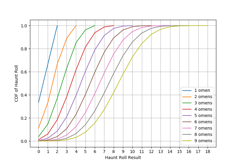
Now that we've gone all the way through this exercise, we can turn to the other versions of the game. Betrayal and Balder's Gate and Betrayal at Mystery Mansion both function similarly (though the latter game uses the term clue instead of omen, it functions the same). Instead of rolling a constant number of dice and adjusting the target number, the number of dice rolled is equal to the number of omen cards drawn and a constant target number is used. In Balder's Gate, if the haunt roll is 6 or higher the haunt starts, whereas Mystery Mansion uses a threshold of 5 or higher.

To compute the distribution of dice, we can use a similar method as above, but varying the number of haunt dice pmfs which are convolved. The resulting pmfs and CDFs are plotted in Figures 4 and 5.

Figure 4: Probability mass function of haunt roll by omen

Figure 5: Cumulative distribution function of haunt roll by omen

We can reuse the same equation to find the pmf and CDF of the number of omens drawn before the haunt starts for the three games, which are plotted in Figures 6 and 7. We can note a couple differences. Most evident is that each iteration on the game tends to make the haunt start sooner, as shown most clearly in the CDFs. Second, the possibility of a very early haunt with the original game, with only 1 or 2 drawn, has been completely eliminated in Balder's Gate and Mystery Mansion. For the later games, rolling one or two dice is insufficient to get a sum or 5 or 6 to trigger the haunt. On the other hand, these games have a non-zero probability of an arbitrarily long game according to the probabilities shown. Mystery Mansion has a special rule that the haunt always starts after the 9th omen (clue) card is drawn.

Figure 6: Probability of triggering the haunt when drawing current omen

Figure 7: Cumulative probability of triggering the haunt

We could modify the dice so that they naturally provide both an upper and lower bound, as originally desired for the spy search mechanism, by using a similar mechanism to the later Betrayal games but having a non-zero minimum value on the dice. Doing this sets a maximum number of turns needed for the search, equal to the ratio between the target sum and the minimum value on the dice.

Recall that we want between 4 and 9 searches, averaging 6-7. Let's use a minimum value of 1 on the dice and decide on the number of values to include to achieve the properties above. With a minimum of 1 and max 9 rounds, the target sum must be 9. To prevent 3 searches from being successful, there must be at most 2 sides on the dice. This gives the distributions functions shown in Figures 8 and 9. While these center more on 6 searches, they demonstrate the feasibility of this type of mechanism. The particular type of dice and target numbers can be adjusted to get the desired probability properties.

Figure 8: Probability of finding the spy in the current round (pmf)

Figure 9: Cumulative probability of finding the spy by round (CDF)